Update 4-11-2022: A version of this information, without all the details, was presented 4-9-22 to the North Houston section of NSS. It was very well-received. The question they posed was using propellant made on the moon to supplement or replace propellant sent up from Earth. I am thinking about how to figure that option. Watch for updates, I may add that.
-------------
ARTICLE
-------------
At the request of some friends and colleagues that I
correspond with, on the New Mars
forums, I have been looking closely at
the propulsion needs and possibilities for sending a very large
orbit-to-orbit transport from Earth to Mars and back, reusably.
We have been calling this the “big ship”. This would be an item that would fly several
years from now, once the beginnings of a
colony effort commence.
Two friends and colleagues have been looking at the concept design
of the transport as a reusable “dead-head” payload item, to be pushed by some sort of reusable propulsion
stage. They have different concepts as
to how to build this item, as indicated
in Figure 1. I have been looking instead
at what that propulsion stage has to do,
and how big it must be, to push
either of these things, or anything else
of a similar nature. One serious problem
is that we still do not know the actual mass of these “dead-head” payload
items. I’m using an assumed value just
to get “into the ballpark”.
The ultimate goal here is a design concept for a ship that can transport up to a thousand people at a time, plus cargo and supplies. It is to fly from low Earth orbit (LEO) to low Mars orbit (LMO) and back. Low orbit basing greatly-reduces the delta-vee (dV) requirements for ferry vehicles, from Earth’s (or Mars’s) surface to orbit and back, to a minimum, something already known to be crucially important.

Figure 1 – Basic Notion Being Evaluated
These are nothing but simple rocket equation
studies, just not done “pencil-and-paper”
with a slide rule, the way I did when I
originally entered the workforce out of college. If you don’t know what a slide rule is, see Ref. 1.
Today’s equivalent is a fully-scientific pocket calculator.
Today, the
calculations have been semi-automated using spreadsheet software, which makes iteration far easier, and errors less likely, plus data can be plotted. Except for that, they really are the same “pencil-and-paper”-type
design analyses of my slide rule days, not
computer models of any kind! This is
2 to 3 significant figure stuff, just
good enough to see the trends. And
trends there are!
This kind of simple equation-based design analysis is not
really taught very much anymore. The
youngsters today jump immediately to this or that computer model, which is exactly what their schooling
studies have emphasized. However, there is considerable effort (and
expenditure) involved in setting up,
de-bugging, and verifying any
computer model, of pretty much
anything. Plus, there are typically only limited variations
you can use the computer model for,
without essentially starting over with a new computer model.
My kind of “pencil-and-paper” design analyses (that I still
do) can usually be done quicker, and
with much less effort, especially given
today’s spreadsheet tools. This
then allows one to screen many different concepts quickly, so that the more extensive (and expensive) finite-element
computer modeling efforts can be concentrated on only the best ideas! That is a very important thing to consider, for cost-effectiveness in your design analysis
effort!
You simply do not need super-precise answers during a fast
concept screen, you only need data just
precise enough to tell the winners from the losers. Later on,
you do need the precision afforded by the computer modeling, once you are fleshing-out a real candidate
design. That distinction is quite
important!
Using the Rocket Equation Properly
Just knowing the rocket equation is a far cry from knowing
how to use it properly for these concept-screening purposes. It was derived for a rocket thrusting in
vacuum under the influence of no outside forces, not even gravity. What it predicts from the vehicle weight
statement and propulsion specific impulse (Isp) is the max
deliverable dV you can expect from that vehicle. It is the weight statement that allows
you to compute the vehicle mass ratio MR,
upon which that dV depends.
Such a weight statement really is just a list of the items, and their masses, that comprise the vehicle burnout mass Wbo, to which you add the propellant mass Wp, to get the vehicle ignition mass Wig. Such lists can vary and be tailored to the
specific application. What is important
are the burnout, propellant, and ignition masses. The mass ratio is then MR = Wig / Wbo, where Wbo + Wp = Wig.
Vehicle dV is computed from the MR with the rocket
equation, using an effective exhaust
velocity Vex for the propulsion. This is
not really the expanded velocity from the engine nozzle exit, although it is usually quite close. It is an effective velocity as if there were
only a momentum term in the thrust equation,
no pressure difference term. It
is particularly easy to compute Vex from the engine specific impulse value
Isp, using a sort of gravitational
constant gc that makes the units consistent.
The need for that is because these definitions preceded the notions of
consistent units-of-measure systems.
The rocket equation itself is deliverable-from-the-vehicle-dV
= Vex LN(MR), where Vex =
Isp * gc.
That deliverable vehicle dV must be compared to a
mission-dependent dV requirement. The
vehicle must be capable of delivering the mission requirement. Or maybe just a bit more, but never less! It must do so despite the effects of both
drag and gravity losses, as applicable
to the mission. Usually, the easiest way to account for such losses is
to take the ideal astronomical dV values,
and factor them up, to larger
“mass ratio-effective” design dV requirements, that your design concept must meet. All
of this is summarized in Figure 2.
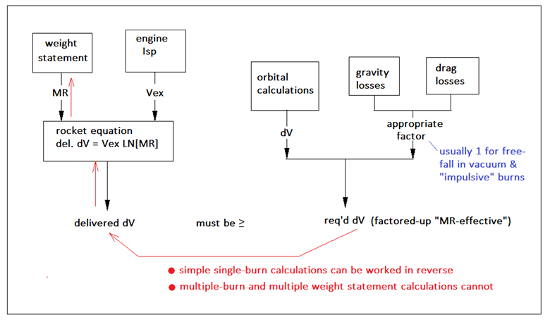
Figure 2 – What Items Are Important to Rocket Equation Design
Analysis
There is a “catch” here:
if all the burns your propulsion must make, take place between the very same Wig and Wbo
values, then you may sum those dV’s into
a single mission dV for purposes of sizing the required overall MR and weight
statement. In effect, you may sum all the dV’s that correspond to a
single weight statement, for design
sizing purposes. The mass ratios
for the individual burns multiply together to become the overall mission mass
ratio. Those individual mass ratios for
each burn may be used to determine the intermediate vehicle masses between the burns, which in turn may be differenced to determine
the propellant used for each burn. This
is illustrated in Figure 3.
On the other hand, if
a payload or inert item changes from one burn to the next, that constitutes a different weight statement
entirely. You cannot sum up dV’s
for burns that use different weight statements. If you do,
you will get wildly-wrong answers.
What you have to do, is a separate rocket equation burn
analysis for each and every dV that has a different weight statement associated
with it. Further, you must do them in the reverse order
of the burn sequence! You must
do it that way, so that the propellants
for the later burns become part of the burnout masses for earlier burns. Fail to get that correct, and once again, you get wildly-incorrect answers. This is also indicated in Figure 3.
The form of the weight statement used for these big ship
studies is particularly simple. There is
the “dead-head” payload mass, and there
is the propulsion stage that pushes it.
That propulsion stage has a total (stage-only) mass that is comprised of
the mass of propellant it contains, plus
some stage inert mass. For this
situation, the vehicle burnout
mass is the sum of the “dead-head” payload mass and the propulsion stage inert
mass. The vehicle ignition mass
is the sum of the burnout mass and the propellant mass in the propulsion
stage. We just need a way to estimate
propulsion stage propellant and inert mass fractions. This is also indicated in Figure 3.

Figure 3 – Impact of One vs Multiple Weight Statements
Associated With Each dV Value
I chose to model this as a propulsion stage-only
propellant mass fraction R. This is
propulsion stage propellant mass divided by propulsion stage-only total
mass. For example, if the propulsion stage total were 100
tons, and its R = 0.97, that means the propulsion stage has 97 tons
of propellant, and 3 tons of inerts. Those inerts would be the tankage, any insulation or coolers that it has, any propulsion or flight controls that it
has, any other equipment that it might
have, and the mass of the engines that
it has. This stage then pushes the
“dead-head” payload item as a combined vehicle, so that the vehicle burnout mass is stage
inert plus “dead-head”.
The rocket equation determines your vehicle’s deliverable dV
value. That must equal or exceed what I
have been calling the “mass ratio-effective mission dV value”. This is the sum (as appropriate) of the
mission astronomical dV values, each factored-up
to account for any gravity and drag losses that might apply.
Determining Mission dV Values
The details depend upon exactly what mission you are trying
to do. The baseline here was low
circular orbit at Earth to low circular orbit at Mars. This could be done as min-energy Hohmann
transfer, or a faster trajectory. One variation is flying the 2-way round trip
unrefilled, vs refilling at Mars before
returning to Earth. Other variations
include the use of an elliptic capture orbit at Earth, Mars,
or both. Ref. 2 is one place
where I looked at determining astronomical dV values for various transfers.
To use elliptic capture,
the assistance of a space tug is needed.
For departure the tug takes the fully-filled “big ship” from low
circular orbit speed to the periapsis speed for the elongated capture
ellipse, which is something a bit under
local escape speed. The tug then
undocks, and the big ship must immediately
thrust from periapsis speed to the required end-of burn speed (which is
something a bit more than local escape speed) while still quite near the
planet. Meanwhile, the now-unladen tug must return to low
circular orbit. See Figure 4 for the dV
data as a function of these mission nuances.
Arrival is similar,
but differs because of inherent timing issues and the lower mass of the
arriving “big ship”. The “big ship”
burns its last propellant entering the elliptic capture orbit at its periapsis
point. The unladen tug waits in low
circular while the big ship makes a turn about the elliptic capture orbit. The tug then fires to enter the elliptic
orbit just as the big ship hits periapsis.
The tug rendezvouses (which takes significant time), and the docked pair must then make another
turn about the elliptic orbit. The now
heavily-laden tug then fires at periapsis to bring the docked pair into low
circular orbit.
The numbers for Earth and Mars are different, so Earth tugs are analyzed separately from
Mars tugs. The “big ship” is much more
massive at departure than arrival, so it
is departure that sizes the fully-loaded tug stage. For arrival,
the very same tug can be used with only a partial load of
propellant. The point here is that
there are 4 burn cases to analyze, each
with a different weight statement, for
an Earth tug (2 burns, 2 weight
statements), and again 4 cases to
analyze for a Mars tug.
The ”big ship” can be analyzed as a single mission-effective
dV within a single weight statement,
even for a round trip, if one
assumes the same “dead-head” mass on return as outbound. Such is the conservative assumption, and that is what I did. There is a dV to depart Earth, a course correction dV along the way, and an arrival dV at Mars. These sum to a 1-way dV. The numbers are higher for the fast
trajectory, of course. You double it for 2-way. “Big ship” dV data are shown in Figure 4B.

Figure 4 – Values of dV Applicable to the “Big Ship” As a
Function of All the Mission Variations

Figure 4B – “Big Ship” dV Data Summed for the Mission Cases
Note that the 30-month Hohmann round trip exceeds the
26-month interval between planetary line-ups to go on such a mission. That means there is 52 months between
successive “big ship” missions, using
Hohmann, which affects required
propellant manufacturing rates. The
fast trajectory is a 2-year abort trajectory,
which is a 24-month mission.
These can be flown every planetary line-up, meaning 26 months between successive
missions. That doubles the manufacturing
rates, all else being equal.
The space tug dV data at Earth and at Mars are given in
Figure 5.

Figure 5 – Relevant dV Data for Space Tugs at Earth and at
Mars
Caution!
There is a double nuance here, that many do not appreciate. One is that there is a change of coordinate
systems from “with respect to the planet” to “with respect to the sun”. The other is the effect of planetary gravity
slowing the vehicle as it recedes from the planet after the burn. That burn takes place necessarily close-in, at the low orbit altitude.
The gravity effect is accounted for, while considering the vehicle velocity with
respect to the planet. After the
burn, the vehicle has a fixed mechanical
energy, that being the sum of its
potential and kinetic energies with respect to the planet. As it recedes, the potential energy increases, and so the kinetic energy decreases. The definition of escape speed is the
velocity “near” such that the velocity “far” is zero. You evaluate escape speed at the low circular
orbit altitude, and “far” is
“infinity”. Thus:
Vnear2
= Vfar2 + Vesc2
where Vesc is figured at the “near” distance
The change in coordinate systems is
accomplished by adding the planet’s velocity vector about the sun to the
velocity vector of the vehicle with respect to the planet, once it is “far” from the planet. That “far” vehicle velocity with respect
to the sun must match the orbital transfer perihelion velocity for Earth
departures, and the transfer apohelion
velocity for Hohmann returns. This is
definitely a vector addition/subtraction for the fast trajectory, where the Mars encounters involve
non-parallel velocity vectors of vehicle and planet, by more than 30 degrees. Scalar math only works when the velocity
vectors are parallel.
One actually works this calculation process in reverse. One determines from the transfer trajectory
and the planetary orbital velocities (with respect to the sun) the needed value
of “Vfar” with respect to the sun, then
the planet. Then one uses the gravity
correction to compute “Vnear”, which is
substantially larger. That is the
required vehicle velocity at end-of-burn for departure, which is conducted “near” the planet. The difference between that, and the appropriate orbital velocity about the
planet, is the required departure
dV. Arrival dV has the same value, it is just that the thrust direction is
reversed.
“Mass Ratio-Effective dV” Factoring
This is a very serious effect for launching from the
surface. There are both drag and gravity
losses to account-for, and they are very, very significant, each being around 5% of low orbital
velocity, here at Earth. That topic is basically out of scope
here, since we are talking about
departures from, and arrivals to, orbits in space about the planets.
For these studies,
all burns and trajectories are out in the vacuum of space, so that there are no drag losses to worry
about. There can still be gravity
losses, if the burn takes a long
time, during which the vehicle’s radial
distance from its primary body increases measurably. That radial distance increase is an increase
of potential energy. Propulsive energy
that goes into increasing potential energy instead of kinetic energy, is “lost” energy as far as the rocket
equation is concerned, it being derived
for no gravitational influence at all.
If the burn is short enough, so that no measurable radial distance increase
occurs during the burn, then there is no
measurable gravitational loss. Such are
termed “impulsive” burns. I use a “rule
of thumb” for that: thrust sufficient so
that vehicle acceleration exceeds something like 0.01 to 0.1 gee. I used 0.05 gee for these studies to size the
minimum thrust requirements for the various vehicles.
The factor is 1 plus the gravity loss expressed as a
fraction of some suitable baseline, plus
the drag loss expressed as a fraction of some suitable baseline. If both losses are zero, the factor is just 1, and the astronomical dV values really are the
mass ratio-effective dV values.
Electric propulsion, as we know it at this time in history, is the “odd case”, because its thrust is but a whisper produced
by tons of machinery and equipment (including a big electric power supply of
some kind). Vehicle accelerations are
far, far less than 0.01 gee. Such is termed “non-impulsive”. There is very significant gravity loss
associated with this. Further, the trajectories themselves are no longer the
2-body elliptical orbits at all. Such
vehicles thrust continuously, following
outward or inward spirals about the primary body. That is true whether the primary is a
planet, or the sun.
The usual way to approximate this for sizing purposes
is to consider what the Hohmann min-energy transfer orbit(s) would be, figure those dV values, and apply a factor to them. For these studies, I used factor = 2 for electric
propulsion. Some others recommend factor
= 1.5, but mine is more
conservative. Better too much propellant
than too little.
How to Get Launch Propellant From On-Orbit Propellant
I have already looked at the potential payload capability of
the Spacex Starship/Superheavy launch vehicle,
to low eastward Earth orbit (Ref. 3).
Although that is based on earlier data and results, it is probably still “pretty close in the
ballpark”. I simply used those earlier
results in my studies here, as the
closest thing contemplated, that might
actually fall in the class of reusable Earth-to-orbit ferry vehicles needed for
a “big ship”. At nearly $2B per
launch, SLS does not qualify as a
practical orbital ferry, nor is it
reusable.
I have also looked at using Spacex’s Starship as a
single-stage orbital ferry on Mars (ref. 4).
Those results are older, and less
certain, but still “ballpark
correct”. I simply rounded the low
eastward Mars orbit payload off to a nominal 200 metric tons, and used that as “representative”.
There are no such large-payload orbital ferries yet
flying, here or at Mars. The Spacex designs are still early in their
development. I just used projected
performances to “get into the ballpark”.
See Figure 6.

Figure 6 – Spacex Designs Used As “Typical” Of Reusable Orbital
Ferries At Earth and At Mars
You can use these ferry-performance numbers in either of two
ways. Both get about the same
answers, expressed in terms of launch
propellant tonnages required to send payload tonnages to orbit.
The first is to divide your total on-orbit propellant requirement
for the “big ship” and any tugs by the ferry payload amount, to get a number of tanker flights. Round this up to the next nearest
integer, and multiply that integer by
the tonnage of propellant consumed by the ferry vehicle to fly each tanker mission. That product is the launch propellant
required for a given on-orbit propellant requirement.
The second is to compute the ratio of propellant consumed by
the ferry vehicle during its mission, to
the payload it can deliver on-orbit. You
multiply your on-orbit propellant requirement by this ratio, to estimate the launch propellant
required, and then round that up
slightly. That is pretty much the same
answer. Remember, this is really only 3 significant figure
stuff!
Launch propellant dominates over on-orbit propellant by
far, especially at Earth, with its deeper gravity well. The sum of launch propellant and on-orbit
propellant is the total propellant (of all types) that you have to manufacture at
each planet to support a single “big ship” mission. That total propellant requirement, divided by the time interval between such
missions, is the minimum manufacturing
rate that you must be capable of, to
support these kinds of “big ship” missions,
again for each planet.
The best way to judge the effectiveness of the various kinds
of propulsion, and any mission nuances
such as space tugs, is to look at the propellant
manufacturing quantities per “big ship” mission, required at both Earth and Mars, and also at the manufacturing rates required at
Earth and Mars. These quantities
and rates determine the propellant-manufacturing infrastructure needed at both
planets, which must be dedicated to
running such missions at all.
The Studies I Ran
The first study looked at chemical, solid core nuclear, and (generic) electric propulsion, as technologies more-or-less ready to apply
for this mission, done as Hohmann
min-energy transfer only. I also looked
at three different gas core nuclear thermal concepts, and the old fission-device explosion
propulsion concept, as advanced
technologies far from being ready to apply,
but with really attractive performance potential. These also were Hohmann transfer comparisons
only.
Except for the chemical,
all propulsion was evaluated in terms of a 2-way round trip single
stage, without any refilling on-orbit at
Mars, and without any space
tugs/elliptic capture orbits. I did not
believe that chemical, as represented by
Spacex’s LOX-LCH4 engines, would be
capable of the 2-way round trip, so I
instead looked at it 1-way, refilled
on-orbit at Mars. Again, this is only Hohmann.
It was only later in the studies that I found out that LOX-LCH4
chemical was indeed just barely technically feasible for a 2-way trip, unrefilled at Mars. Those results got added later, but I added them to the results here. The storable propellants at Isp ~ 330 s are just
not capable of the 2-way trip single stage,
while LOX-LH2 at Isp > 460 s is.
That’s the Isp effect in action.
The limiting Isp is actually pretty close to LOX-LCH4’s Isp ~ 380
s, for Hohmann transfer and low-orbit to
low-orbit missions. I used an arbitrary
propulsion stage-only propellant mass fraction estimate of 0.97 for these
calculations.
For solid core nuclear, I used the 1974-vintage results from NERVA. This was developed during old Project
Rover, and was ready for its first
experimental flight test, when the
project was shut down. On-orbit
propellant requirements are still high,
but not nearly as high as chemical. That’s the effect of roughly a
factor of 2 higher Isp. I modeled the
heavier reactor core in the engine by reducing propulsion stage-only propellant
mass fraction to 0.95.
“Generic” electric is a flying technology, but has yet to be scaled up to the really
large thrusts and electric power levels that a “big ship” propulsion stage
would require. This is a more-or-less
ready to apply technology, but is not
yet “off-the-shelf” at this scale. I had
to factor-up the Hohmann dV data to model this realistically (factor = 2), and I lowered the propellant mass fraction of
the propulsion stage-only, to 0.90, to reflect the extra mass of the required
large electric power supply. One can
always argue about my specific choices for these factors, but I believe them to be at least “ballpark
correct”.
The gas core nuclear thermal concepts divide into 3 separate
types: the closed-cycle “nuclear light
bulb”, the power-limited open-cycle that
needs no waste heat radiators, and the
high-power open-cycle that does require large,
massive waste heat radiators. All
of these are speculative paper designs,
with only some bench-top experiments that support them. Most of my numbers trace to the proposals
authored by Maxwell Hunter at United Aircraft/Pratt & Whitney in the
1960’s. I used propulsion stage-only
propellant mass fractions of 0.95 for all of them but the high-power gas
core, which has to have such large, heavy waste heat radiators. I used propellant mass fractions between 0.50
and 0.75 for it.
The fission explosion drive traces to old USAF Project
Orion, circa 1959-1965, conducted at General Atomics in San
Diego. The numbers are well-supported by
calculations, plus a subscale
demonstration of explosion propulsion with a 1-meter scale model driven by
high-explosive charges, and the
survivability results for massive steel structures, from the atomic tests in Nevada in the
1950’s.
I probably did not penalize it enough for propulsion inert
mass at a “propellant” mass fraction of 0.90.
That propellant mass would be the mass of all the small fission charges
used in the pulsed “burns”. Those are
effectively shaped-charge nuclear explosives,
with a vaporized reaction mass intended to impact the “pusher plate”, in the design.
This explosion drive technology is probably the closest to
being made “ready-to-apply” of all of the speculative gas core concepts, but it does still pose some severe challenges
to resolve. Perhaps the most difficult
challenge will be the electromagnetic pulse (EMP) effect of nuclear explosions
in low orbit, as demonstrated by the
1962 “Starfish Prime” nuclear detonation in space, above Johnston Island.
The first study results showed enormous propellant
quantities required on-orbit by chemical,
and to some extent by NERVA, with
electric looking fairly good. The still
quite-speculative gas core nuclear and explosion drive options looked really
good, by comparison. See Figure 7.
Those results do not include the propellant needed to launch these
on-orbit propellants into orbit. Those
are given in Figure 8.

Figure 7 – Results From the First Study Excluding Chemical
2-way: On-Orbit Only
The chemical scenario which later proved to be barely
technically feasible, was 2-way
single-stage with no refill at Mars,
from low Earth orbit to low Mars orbit,
and back, with no space tug
assistance. This was the very worst
case, in terms of propellants required
on-orbit, for launch and total propellant
quantities per mission, and for required
manufacturing rates per month. See Figure
9, a later result.
The next-worse case was chemical with a 2-way “big ship”
unrefilled at Mars, but assisted by a
space tug at Earth for its arrivals and departures there. That made a huge difference, although the numbers are still enormous, as indicated in Figure 10. That case still requires no propellant
manufacturing infrastructure at Mars.
All the other chemical scenarios do. This is also one of the later results.

Figure 8 – Gross-Estimated Launch and Totals and Rates for
the First Study, Excluding Chemical
2-way

Figure 9 – Results For Chemical 2-Way With No Refill At
Mars, No Tugs At Either Planet

Figure 10 – Chemical 2-way “Big Ship” Unrefilled at
Mars, But With Tug Assistance At Earth
Bear in mind that the ferry vehicles serving as tankers are
always presumed to be chemical propulsion,
in particular the same LOX-LCH4 propulsion of the Starship and
Starship/Superheavy launch vehicles.
This is to prevent any possible risks of surface or atmospheric
radioactive contamination with the nuclear propulsion options. Electric as we currently know it is quite
simply technically infeasible as a launch vehicle from any planetary surface
whatsoever, and from most larger
asteroids. The thrust is just too
low, compared to any possible vehicle
mass.
The second study looked only at chemical
propulsion (as represented by LOX-LCH4),
but it evaluated the effects of space tugs and elliptic capture at
Earth, at Mars, and at both planets, on a 1-way big ship always refilled at Mars. These mission nuances made a huge difference
in total propellant quantities and rates,
at both Earth and Mars! See
figures 11 and 12. For this kind of propulsion, having space tugs at both Earth and Mars
looked best, by far.
The third study looked at using NERVA solid
core nuclear thermal propulsion with the elliptic capture / space tug mission
nuances considered, but only for Hohmann
transfer. As with chemical, this use of tugs made a large
difference. Space tugs at Earth
only, and at both Earth and Mars, were the best options, and roughly equal. Those tugs use the same NERVA
propulsion! Chemical propulsion, specifically LOX-LCH4, is presumed for the ferry/tanker craft. There is less infrastructure to be created
on Mars with the Earth-only tug approach,
so this was recommended as “best”.
See figures 13 and 14.

Figure 11 – Quantity Results for Chemical “Big Ship”
Hohmann, 1-Way Refilled At Mars, With Tugs

Figure 12 – Rate Results for Chemical “Big Ship”
Hohmann, 1-Way Refilled At Mars, With Tugs

Figure 13 – Quantity Results for the NERVA Study, Hohmann,
2-Way vs 1-Way, and Tugs

Figure 14 – Rate Results for the NERVA Study, Hohmann,
2-way vs 1-Way, and Tugs
The fourth study looked at the high-power gas
core option, as either 2-way or 1-way
designs, and with both Hohmann
min-energy transfer, and with faster transfer
on a 2-year abort trajectory. Elliptic
capture and space tugs were not investigated,
since the propellant quantities and rates were already so attractively
low, regardless. See Figures 15 and 16.

Figure 15 – Quantity Results for
High-Power Gas Core Study, Hohmann vs
Fast, 2-Way vs 1-Way

Figure 16 – Rate Results for High-Power Gas Core Study, Hohmann vs Fast, 2-Way vs 1-Way
One should note that the current Spacex concept for a
Starship returning to Earth from Mars,
requires making some 1200 metric tons of propellant, over the course of roughly a year. That’s in the vicinity of 100 tons per
month.
How I Did It, And
Trends Seen
The core concepts are shown in Figure 17. The equations used, must be used in a sequence. What you do with those equations depends upon
whether you are generating trend plots,
or specific sized-vehicle mass numbers.
The latter is an iterative process,
the former is not.

Figure 17 – Basic Models Used For These Studies
One starts with a mission in mind, and a proposed propulsion concept with which
to do that mission. For it, there are astronomical dV’s, which may need to be factored. For the propulsion, you need to characterize an Isp and a
propulsion stage-only propellant mass fraction R. This propulsion pushes a dead-head payload
item of mass Wdhp. My “figure of merit”
FOM = Wp/Wdhp, which measures tons of
propellant required to push each ton of “dead-head” payload mass, over any particular mission, as modeled by a dV value. I did the studies using the raw variable
format of the equations. However, the normalized version is slightly easier to
scale to other values of “dead-head” payload.

Both of these create exactly the same-shaped plots for a
sequence of user-input Wp values from small to large; the raw variable plot abscissa is Wp, while the normalized variable plot abscissa
is FOM = Wp/Wdhp. If you normalize, you no longer need to pick a specific Wdhp to
create the plots, as long as your R value
is appropriate for a stage pushing a large dead-head item. The influence of different mission nuances
(such as refill and tug assistance) can be large, as shown in Figure 18 and Figure 19.

Figure 18 – Chemical Propulsion Results in Raw Variable
Format, Plotted As Trends

Figure 19 – Chemical Propulsion Results in Normalized
Format, Plotted As Trends
What is going on here is that the stage-only
propellant mass fraction R limits the max achievable values of mass ratio MR. This shows up as a knee in the curve, from a very steep slope, to an essentially flat (zero) slope. You must be operating left of the knee in
the curve, in order to benefit from
large changes in MR for small changes in added propellant quantity. Right of the knee in the curve, enormous changes in added propellant quantity
produce little or no change in achievable mass ratio.
The natural logarithm of the achievable mass ratio, multiplied by the effective exhaust velocity
Vex, is the achievable dV value for the propulsion
stage-plus-“dead-head” payload, as a vehicle. These dV curves reflect exactly the same
shape with a knee, but the levels
achievable reflect the influence of propulsion Isp, which is what sets Vex.
At lower values of Isp,
the relative effects of Isp and R are comparable, while at higher levels of Isp, the value of Isp dominates by far. The “breakpoint” for this, is in the vicinity of 1300 s Isp. Figures 20 – 26 show this, conclusively.

Figure 20 – Curves for LOX-LCH4 Chemical, Use Isp = 380 s and R = 0.97

Figure 21 – Curves for LH2 NERVA, Use Isp = 800 s and R = 0.95

Figure 22 -- Curves for LH2 Nuclear Light Bulb, Use Isp = 1300 s and R = 0.95

Figure 23 -- Curves
for LH2 Gas Core Regeneratively-Cooled,
Use Isp = 2500 s and R = 0.95
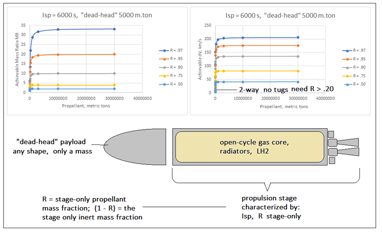
Figure 24 -- Curves for LH2 Gas Core Radiator-Cooled, Use Isp = 6000 s and R = 0.50 to 0.75
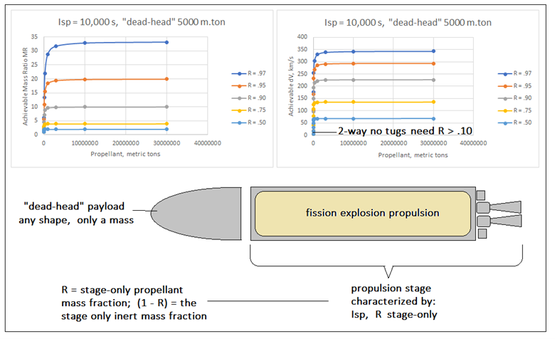
Figure 25 -- Curves for the Fission Explosion Drive, Use Isp = 10,000 s and R = 0.80 to 0.90

Figure 26 -- Curves for the Generic Electric Thruster, Use Isp = 3000 s and R = 0.80 to 0.90
The way to find precise values for a sized vehicle and
propulsion stage is user-iterative.
This is easily done as a spreadsheet.
You input a propellant, compute
from it a stage-only inert mass, add
that propulsion inert to the ”dead-head” payload mass to get a burnout
mass, and add the propellant to that to
get an ignition mass. That weight
statement and Isp get you a vehicle-delivered dV. That delivered dV must equal or slightly
exceed the factored mission astronomical dV.
You iterate the values of
the input propellant until the delivered dV meets the requirement, to the desired precision.
For the “big ship” using one weight statement, that looks like the spreadsheet image in
Figure 27. For the tugs, there are multiple burn calculations at each
of four different “dead-head” payload values (one laden, the other not, and with or without the full propellant load), and at each of the two planets. That looks like what is imaged in Figure 28.

Figure 27 – Image of Spreadsheet Calculation for “Big Ship”
(1-way with Earth & Mars tugs)

Figure 28 – Image of Spreadsheet Calculations for Tugs at
Earth and at Mars (with 1-way big ship)
If you look closely at Figure 27, you can see that the dV requirement
corresponds to tug assist at both Earth and Mars. That applies to both arrivals and
departures, although the event sequence
is slightly different for arrivals. Big
ship Wp numbers were input iteratively until the 1-way surplus was reduced to a
fraction of a meter/second. There is
only the one calculation, because all
three burns (departure, course
correction, and arrival) take place
within the one weight statement. I
simply used this very same result for the journey home, under the assumption that the “dead-head”
payload item is the very same 5000 metric tons as outbound.
What Figure 28 shows for the tugs is four separate
calculation blocks, each with two burns
in it. There is a departure calculation
block on the left for departure, and an
arrival block on the right. The upper
two are for the Earth tug, and the lower
two are for the Mars tug (different because the dV requirements are different). Departure sizes the tug vehicle at either
planet, including its inert mass, while all that the arrival block does is
figure out what partial load of propellant works with the reduced “dead-head”
payload + stage mass, depleted of
propellant after entering the elliptic capture orbit.
In the departure blocks,
the first burn calculated is the second burn in the sequence, which is the return of the unladen tug to low
circular orbit. The second burn
calculated is the first burn in the sequence,
which is pushing the “dead-head” payload from circular to elliptic
capture periapsis speed. Both burns
comprise the astronomical dV circular-elliptical, plus a small budget for rendezvous. The “dead-head” payload is at its max mass
(fully loaded with propellant) during these departure tug assist
operations. That’s what really sizes the
tug.
In the arrival blocks,
the first burn calculated is the second burn in the sequence, which is pushing the “dead-head” payload from
elliptic to circular orbit. The second
burn calculated is the first burn in the sequence, which is the unladen tug moving from circular
to elliptic orbit, to meet the big
ship. The “dead-head” payload + stage is
at its min mass for these arrival operations,
with its propellant depleted from the arrival into the elliptic capture
orbit. No second tug design is required
for this, you just determine a
less-than-max propellant load in the tug that was actually sized for departure.
The unladen tug burns for departure and arrival actually
share the same weight statements, and
mass ratios, which is why those two Wp
values work out to the very same values.
Nothing else about the tug is the same,
though.
You get something “reasonable” into the smaller unladen burn
in the departure block, then iterate to
convergence with the fully loaded burn.
Then go back and iterate to convergence with the unladen burn. Then return
and iterate to convergence again with the fully loaded burn. Most of the time, that’s all you need to do. Sometimes you need another iteration cycle of
both burns, to get “close enough”, which is some fraction of a meter/second in
the total dV required of each burn.
Then load your same unladen propellant quantity in the
unladen burn propellant for the arrival block.
Then iterate the fully-loaded propellant to convergence. Most of the time, that is all you need to do. Sometimes,
another iteration cycle of both burns is needed to get “close
enough”, but that is rare. So also is the unladen propellant quantity
being any different from departure quite rare.
Totaling It All Up
What you have done is calculate the big ship and tug
propellant requirements needed on-orbit at both Earth and Mars. Be sure to add up both the departure and
arrival propellants for the tugs, plus
big ship. Now, estimate the launch propellants needed to
orbit all of those propellants, at both
planets, per the descriptions already
given above. Add the on-orbit and
launch requirements to create manufacturing quantity totals for a mission, at both planets. It may or may not be the same
propellant, but with chemical
launch, the launch propellants dominate
this picture, and by far, especially at Earth.
Manufacturing minimum rates depend upon the interval between
missions. The planets line-up for a
mission from Earth to Mars every 26 months.
Hohmann transfer is on-average a 30-month mission, meaning you can send the same big ship back
on another mission only every other line-up.
That’s 52 months between missions.
The fast transfer using the 2-year abort is different: that mission is a 24-month mission, with about the same year’s stay at Mars, between where you get off the transfer, and where you get back on to go home. You can therefore fly one of these fast
missions every 26 months, which acts to
double the manufacturing rate requirements over Hohmann transfer, everything else equal. Divide your total quantities by your interval
to compute that min required manufacturing rate, at each planet.
Which Is Better?
Raw Or Normalized?
If you compare Figure 18 with Figure 19, you can see that they tell exactly the
same story. Which shows that the
normalized format is a perfectly-acceptable way to explore such
possibilities. You do not have to
actually pick specific values of “dead-head” payload Wdhp and stage propellant
Wp to use the normalized format, only
appropriate values of the figure-of-merit FOM = Wp/Wdhp. I set up the spreadsheet before I knew about
this issue, in the raw data format. If I had it to do again, I’d probably use the normalized format. It’s very slightly easier to scale to other
“dead-head” payload values.
The other thing either of these figures (or Figures 20-26) show
is the enormous impact that mission nuance details can have on the stage
sizing results! Remember, you not only want to be left of the knee in
the curves, you also want to be as far
down toward the origin as possible, in
order to minimize propellant requirements.
What is barely technically feasible up near the knee is very unlikely
to be economically feasible, much less economically
attractive. The closer to the
origin, the better!
This is crucial,
because it costs so very much launch propellant to send these
orbital transport and tug vehicle propellants into orbit at both Earth and Mars. This is especially true at Earth because of
the much deeper gravity well, requiring
multi-stage launch vehicles as the tankers.
With the higher-Isp gas core nuclear, electric,
and explosion propulsion, the
unassisted, unrefilled baselines are so much
lower down toward the origin, that the
refill-at Mars and tug-assistance nuances make far less difference to the
outcomes. Tugs still help with solid-core
NERVA at 800 s Isp (see again Figure 21),
but the effect is almost lost in the noise for the nuclear light bulb
and “hotter” concepts, at 1300+ s Isp
(Figures 22-26).
It Is Your Choice As To Which Format To Use
One can use either the raw-variable or normalized equations
to size a propulsion stage for the big ship,
and any tugs, with the same basic
equation sequence shown above. The
difference is in iterating a single propellant quantity Wp or FOM to converge a
delivered dV with required factored mission dV,
versus just listing some propellant values Wp or FOM to create a visually-informative
plot.
For a single or multiple burns on a single weight
statement, there is but one
iterative calculation to make, toward
the sum of the dV’s. For a change in
weight statements between successive burns,
each burn must be computed separately with its appropriate weight
statement, and in reverse sequence
order, so that the propellant for later
burns is effectively part of the burnout mass for earlier burns. Using the raw-variable format, this is what the “big ship stuff” spreadsheet
does, in the worksheets “ballpark” and
“ballpark tug”. (I could easily re-write
the spreadsheet to use the normalized equations.)
One Last Point:
Any “big ship” and space tug designs of current and
near-term technologies are going to be involved with extensive on-orbit refilling
operations; very extensive indeed, if these numbers are any guide. This would be need to be done from an
on-orbit fuel depot facility somewhat similar to the one depicted in Ref.
5. Doing the “big ship” as a “dead-head”
payload item with a separatable propulsion stage allows the same kind of spin
ullage solutions as are described and recommended in Ref. 5, for the propulsion stage, and any tugs.
The always-spinning “dead-head” payload item then does not impact
refilling, because the propulsion
stage is separable.
This solution is obviously advantageous for LEO, where the quantities are so much larger. It is not required, but it would be desired, for handling the smaller quantities involved
with refilling in LMO. Planning to
construct such a facility in LMO is thus recommended for any long-term
colonization effort.
Conclusions and Recommendations for Earth-Mars Orbital
Transport Design Concepts So Far
1.
If using chemical propulsion with Isp < 500
s, consider carefully
using either refill at Mars, or
assisting tugs, or both, as mission nuances to drastically lower
required factored mission dV’s, relative
to technically-feasible dV’s from the propulsion stage(s). If you don’t,
your mission will prove economically infeasible due to truly enormous
launch propellant quantities, and
possibly even technically infeasible, if
your propulsion stage-only R value is too low.
2.
If using the 1974-vintage NERVA propulsion at
Isp = 800 s, you are much further away from
any technical infeasibility, yet
the nuances of refilling at Mars, and/or
assisting with tugs, are still quite
significant and very beneficial.
It makes sense to use the same NERVA propulsion in the tugs as in the
“big ship” propulsion stage, but for
safety’s sake to use chemical propulsion for launching propellants to orbit.
3.
If using anything equivalent to the nuclear
light bulb at 1300 s or higher Isp, mission
nuances like refill at Mars and tug assist become far less important, even to economic feasibility with chemical
launch of propellants to orbit. The only
thing currently flying in that range of performance is electric propulsion
(requiring factoring up the astronomical dV’s because these are non-impulsive
burns), and electric propulsion tugs are
not feasible: they must provide
impulsive burns! You therefore must use
a high-thrust propulsion concept in your tugs,
if you try to use tugs with an electric propulsion big ship. I have not looked at that option yet.
4.
Intense development of the gas core nuclear and the
nuclear explosion concepts, is very most
certainly warranted, in order to have
something besides, and likely better
than, than electric propulsion for this
mission.
5.
Consider using an on-orbit propellant depot for
low orbit refilling operations, especially
at Earth, and likely at Mars.
References
For articles posted on the “exrocketman” blog site, use the navigation tool on the left side of
the page. Click on the year, then click on the month, then click on the title if need be.
#1. G. W. Johnson,
“THIS is a Slide Rule!”, posted
16 March 2019, on http://exrocketman.blogspot.com
#2. G. W. Johnson,
“Fundamentals of Elliptic Orbits”,
posted 5 March 2021 on http://exrocketman.blogspot.com
#3. G. W. Johnson,
“Reverse-Engineering Starship/Superheavy 2021”, posted 9 March 2021 on http://exrocketman.blogspot.com
#4. G. W. Johnson,
“Spacex Starship as a Ferry For Colonization Ships”, posted 16 September 2019 on http://exrocketman.blogspot.com
#5. G. W. Johnson, “A
Concept For an On-Orbit Propellant Depot”,
posted 1 February 2022 on http://exrocketman.blogspot.com
Postscriptum:
These results, at the
scope and definition presented herein,
are scheduled to be presented at a meeting of the North Houston ISS
chapter, on 9 April 2022. Meanwhile,
the notion of an electric propulsion “big ship” assisted by
chemical-propulsion tugs at only Earth,
seems attractive enough to investigate.
Watch this space for any updates.
Update 5-14-2022: That presentation resulted in a question about propellant supplied from the moon instead of from Earth. I looked closely at that. I wrote a new article describing those results. It was posted 1 May 2022 as "Investigation: "Big Ship" Propellant From The Moon vs. From Earth". That option proved to be quite effective.
