Update 10-6-15:
For an E-85-type ethanol conversion, there are 3 things you must address: (1) mixture ratio at all power settings, (2) extra timing advance, on the order of 15 extra crankshaft degrees, and (3) quite a bit of extra intake heat to promote adequate vaporization.
If you plan on burning something more concentrated than E-85, there is a fourth item: (4) you will need a start fuel canister of some kind. Otherwise starting at ambient temperatures below 50 F becomes essentially impossible.
For a stiff blend up to E-35, there is no conversion at all! It is just a drop-in fuel. And ethanol splash-blends with gasoline in the tank, so stratification isn't an issue at all. With today's E-10 for unleaded regular grade, use no more than 1/3 E-85 by volume, no less than 2/3 regular by volume, and your mixture will be no stronger than E-35. If it takes 12 gallons to fill up, no more than 4 of those should be E-85, no less than 8 of those should be unleaded regular.
Full E-85 conversions: Mixture Ratio -- With carburetors, increase main jet and idle jet sizes by roughly about factor 1.2 on diameter. You have to sneak up on the right value, it is different for every car. For fuel injection, replace the fuel rail pressure regulator with an adjustable aftermarket unit and set it about factor 1.5 higher pressure, and do not tell the electronics you did anything at all.
Full E-85 conversions: Extra Timing Advance -- First thing to try is +15 crankshaft degrees from gasoline stock. Ethanol's burn speed is similar to gasoline, but its ignition delay is longer so you must start earlier with your spark. What you want to end up with is peak cylinder pressure 1-2 crankshaft degrees before top dead center, no more, no less. This issue is extremely serious with a modern over-square, short-stroke, high-rev automotive engine. With very old under-square, long-stroke, slow-rev technology, this issue makes almost no difference at all.
Full E-85 conversions: Extra Intake Heat -- it is impractical to modify the intake manifold hot spot in most engines. The only viable alternative is hotter intake air. It needs to be above about 70-80 F minimum, before fuel is introduced. 90 F is even better.
Original Article:
Some folks have contacted me for help do-it-yourself converting cars to E-85 or for using "stiff" gasohol blends in unmodified cars. Here's what I know works ----
"Ethanol VW"
My "ethanol VW" was a 1973 beetle with an essentially-stock 1600 cc case, jugs, and crank. It was a dual-port head engine, stock valves, stock rockers, no modifications at all. I had long ago replaced the worn-out combination distributor with an aftermarket Bosch 009 all-mechanical unit. (I had also long ago undone the idiot 15-degrees-retarded timing setting, that the factory used in 1973 to try to meet EPA emission standards. This took me from 5 degrees late (mark on pulley) to 10 degrees before top dead center, static timing.)
After I got the Bosch-009, what worked best for ignition timing was a very simple 30 degrees all-in (about 2500+ rpm) by strobe, on gasoline. I used this setting successfully for decades. I decreased the valve lash setting and oil change intervals to 2000 miles from the factory-recommended 3000 miles, and changed from the recommended lash of 0.006 inches intake and exhaust to 0.006 inch intake and 0.008 inch exhaust. These changes enabled me to avoid valve-burning and excess bearing wear problems in the Texas heat. By switching to aviation-grade oil in the 1980’s, I was able to increase the oil change interval to 4000 miles. After the advent of SF-or-better grade auto oils in the mid 1990’s, I was able to return to using auto oils at the longer 4000 mile interval.
The original carburetor was a Solex 34 PICT-3. I went through a couple of them; they wear around the shaft of the throttle plate, and leak air. It upsets the off-idle transition very badly. I had finally replaced it with an aftermarket Solex 30/31 with the adapter plate for the 34 mm manifold. That worked fine for many years, but finally wore out the same way as the 34 PICT-3. I also had available, but had never used, a not-worn-out Solex 30-PICT-2, off a single port head 1600 cc Bus engine.
I went through several combinations of jet sizes with both the 34 PICT-3 and the 30 PICT-2 carburetors, before I settled on the 30 PICT-2, because it did not leak air around the throttle butterfly shaft. I had to use the adapter for the 30/31 to make it fit, and the accelerator pump cover off the 30/31, to find an accelerator pump link bar that would fit. I never even tried the 30/31 with ethanol, because it has idle circuitry that I never really understood: it uses two idle jets of different sizes.
The Converted 30 PICT-2
On the 30 PICT-2 the stock main jet was a "116.0", which is 1.160 mm dia (.045"). On E-85, I settled on a "137.5" from another aftermarket Solex-Brazil carburetor, which is 1.375 mm dia (.054") for good driveability at speed. The stock idle jet was a g55, which is 0.055 mm dia (.022"). I drilled that out to .762 mm (.030") before I was satisfied with idle settings. If the idle jet is too small, you will suck the idle well dry with too much idle circuit air flow, because the idle screw is open too wide. It's a transient effect, with a time constant somewhere around 15-30 seconds. The stock accelerator discharge nozzle is right at .50 mm dia (.020"). I drilled that out to .712 mm dia (.028") before I was satisfied with the off-idle transition.
Ignition Timing Changes
None of this works at all, if you don't first revise the timing. I found that out the hard way. On gasoline with my aftermarket distributor, timing was +30 BTDC all-in at about 2500+ rpm. I set that with a strobe as the most repeatable way. I had to add 15 degrees to that setting, before it showed the same coast-down vacuum curve on E-85. On E-85, the revised timing spec was thus +45 degrees BTDC, all-in at 2500+ rpm. In other words, you need to add right about 15 crankshaft degrees to whatever timing setting you are using on gasoline. Use the minimum that recreates your old gasoline vacuum coastdown curve.
The Converted 34 PICT-3
You may still have a 34 PICT-3 carburetor. If so, here are the best jet combinations I found, before I gave up on it due to the shaft air leak. Stock main is a "127.5", which is 1.275 mm dia (.050"). On E-85, I used a drilled-out 1.57 mm dia (.062"). Stock idle was a "g55", which is 0.55 mm dia (.022"). On E-85, I drilled that out to .965 mm dia (.038"). Stock accelerator discharge was 0.50 mm dia (.020"). On E-85, I drilled that out to .965 mm dia (.038"). I give both metric and US sizes, because it's a metric car, but all I had to work with was a set of the tiny US-sized bits one uses to clean out oxyacetylene torch tips.
Heated Intake Air
The only other thing I had to do (which you might not if it never gets cold where you are) was to fool the intake air into thinking it was always summer. Any time the outside air temperature was under 70 F, I sucked my intake combustion air from a partial sheet metal glove around the muffler, made from scrap metal roofing trim. Above 70F, ambient air works fine. If you don't do this, both driveability and mileage suffer whenever it is cold. This rig worked all the way down to 15 F for me. I did it with a tee made of scrap plastic bottles on the air cleaner intake. I just plugged-up the cold inlet in cold weather, and let it draw from both inlets in warm weather. My hot source was connected to the side inlet of the tee, which has just a tad more flow resistance. Thus it favored cold air with both inlets open.
How It Should Perform
Have fun running your late-model 1600 VW beetle (or bus) on E-85. If you do it right, you should get about 80% of your former gasoline mileage, not the 70% that the fuel energy per gallon says you should get. Ethanol simply burns more efficiently than gasoline in a piston engine. This partially offsets the lower energy per gallon of the ethanol. Tailpipe soot should gradually disappear. Your spark plugs will start looking pristine-clean, too. So also will the carburetor casting look much cleaner, inside and out. It's really amazing how much cleaner E-85 is than gasoline, in so many different ways.
Minor-to-Moderate Compression Troubles, and How to Cope
If you smell ethanol in your motor oil (it'll smell different, anyway, so I am talking about detecting really serious odor here), your rings are leaking. This will show up as uneven (by around 15 psi) or generally somewhat-low (by about 15 psi) dry compression test readings. If your readings are worse than that, you really need to do the overhaul work first. Add about 10 or 20% Lucas Oil Stabilizer to your crankcase oil, and that modest compression defect will correct itself, and the fuel smell in the oil will go away.
Use the "finger test" to reset your oil change interval, it'll get substantially longer with synthetic in the mix like that (mine pretty much doubled from 4000 to at least 8000 miles, on modern SM-rated oils in an 80-20 blend). The Lucas additive really does a good job arresting cold start wear. Before the advent of SF-grade oils, I could not get even 3000 miles without seriously failing the finger test, so I used aviation-grade oils instead. Nowadays, the SM-grade(same as ILSAC-4, by the way) is way better than the aviation grade oil.
If you don’t understand how to run the “finger test”, you better ask me, or a professional mechanic. It’ll tell you everything a lab test can tell, except for a numerical particle identity and count. But, if you see visible metal wear particles, that’s all you need to know anyway (time to overhaul completely).
Carbureted “Flex-Fuel”?
My 1973 VW beetle is going back into mothballs. Before I was done with it, I reset the carburetor back to gasoline settings by installing a screw on the enlarged main jet, reset the timing back to gasoline-suitable, and undid the heated intake air. I didn’t change the enlarged idle or accelerator discharge. I just reset the idle speed and mixture screw settings as needed, to make it run just fine on gasoline. Then I ran progressively-stiffer gasohol blends until I saw the late timing problem kick-in about E-45-ish on blend strength. The car ran just fine testing blends all the way to E-57 like that. I got the same story (late timing above about E-45) from fuel mileage figures in my fuel-injected unmodified 1995 F-150, and subjectively from my fuel-injected, unmodified 1998 Nissan Sentra.
I did have to reset the VW carburetor screws a little for the blends above about E-40. The fuel-injected Ford and Nissan needed nothing at all, all the way to E-50-something (because closed-loop injection compensates mixture strength automatically, within system flow rate limits).
The requirement for the extra 15 degrees of timing advance (and presumably the warmed intake air) seems to kick-in like a light switch, right about at E-45-ish. If you don’t make these changes, then above E-45-ish, you run weak, smooth, and fuel-consumptive, with a little less intake vacuum on coastdown. That's symptomatic of late timing.
Blend Limits for Unmodified Engines
Cold-weather start "irritations" limited me to E-30 to E-35 max in the unmodified fuel-injected cars. These take the form of starting but dying quickly. A second start then usually works just fine. The problems kick in about freezing. I have tested down to about 10 F here in Texas. This is not serious, just irritating. I have a very old carbureted VW beetle (1960 model) that is running totally unmodified on E-34, and it seems to be doing OK, too. All my completely-unmodifiable lawn and garden equipment runs just fine on E-34, and has for 4 years now.
E-85 is nominally 85% by volume ethanol and 15% gasoline. Its nominal volume fraction ethanol is thus 0.85. These days, unleaded regular gasoline is nominally 10% by volume ethanol and 90% gasoline. Its nominal volume fraction ethanol is thus 0.10. If you know how many gallons of fuel it takes to fill your tank or fuel can (V), and what blend fraction ethanol you want (R), you can use these figures to compute how many of the fill gallons should be E-85 (X):
X = V / [1 + (0.85 – R) / (R – 0.10)]
Examples: for a desired E-35 blend, R = 0.35. Thus X = V/[1 + .50/.25] = V/3.00. Similarly, for R = 0.30, X = V/3.75. For R = 0.25, X = V/5.00. For R = 0.20, X = V/7.50.
Assuming the tank is burned down pretty low (or the can is nearly empty), the residuals will combine with your fill blend pretty close to the R you selected for the fill. In the case of a vehicle fuel tank, this presumes that you have calibrated your fuel gage for gallons-to-fill versus marks on the gage.
This stuff “splash-blends” right in the tank or fuel can. No mixing is required. Just put in your “X” gallons of E-85, and top-off “to the mark” with gasoline. Total gasoline added should come out very close to “V – X” if you did it right.
Calibrating a Fuel Gage
Keep a mileage log over at least three tankfuls of fuel. Record as a minimum the odometer reading and the gallons-to-fill at each fill-up. Fill the tank to exactly the same mark each time. The average mileage between fill-ups is the difference in odometer readings divided by the gallons-to-fill.
While driving on each tank of fuel, as the gage’s needle reaches each mark on the gage, record that odometer reading. The differences in these recorded readings give you miles-between-marks for that tank of fuel. Dividing those by the average mileage for that tank gives you gallons-between-marks. These you average over the multiple tanks of fuel. Listing the averaged gallons-between-marks in a cumulative fashion gives you gallons-to-fill (V) for each gage mark.
Checking Blend Strengths Experimentally
I do this with a simple added-water phase separation test. This requires lab-grade glassware, those being a graduated cylinder of 100 cc capacity for the fuel sample, and a graduated cylinder of about 30 to 50 cc capacity for the added water. You must “abuse” standard laboratory practice and read these to the nearest quarter-division instead of the standard-practice nearest half-division. If you do it this way, your results will come out pretty close to plus or minus 1 or 2 percentage points on blend strength (plus or minus 1 or 2 E-number points). Smaller sample sizes do not work out accurate enough to be useful. I draw my samples from the Schrader fitting located on the fuel rail in most fuel-injected vehicles.
Draw a fuel sample between 58 and 68 cc in volume into the larger cylinder and measure it precisely (bottom of meniscus, or BOM). Compute 1/3 of this volume for the water, put about that much into the smaller test cylinder, and measure what you have precisely (BOM). Record these numbers. Then add the water to the fuel, which will begin to phase-separate immediately. Let this stand 2-4 minutes until all the air bubbles quit decanting. Then measure the total liquid volume (BOM), and the volume below the interface between the separated layers (there is no meniscus, this is a flat plane).
Now, all the water and the ethanol go to the bottom layer, which may grade from cloudy white below to clear right at the interface. The hydrocarbon will all go to the top layer, which is a clear straw-colored liquid. You cannot use the water-plus-ethanol volume directly, because mixed ethanol and water volumes are not conserved, while mixed ethanol and hydrocarbon volumes are conserved.
Subtract the wet ethanol layer volume from the total separated sample volume to determine the hydrocarbon volume floating on top, and record it. Subtract this hydrocarbon volume from the original fuel sample volume, to determine the wet ethanol volume present in the original fuel sample, and record it. Dividing this wet ethanol volume by the fuel sample volume determines the wet ethanol fraction in the original fuel, which in percentage format is a really good estimate of the blend E-number.
I typically find the E-10 “gasoline” to be really closer to E-8; indeed, the placard on the pump usually says “up to 10% ethanol”, not “exactly 10% ethanol”. E-85 typically tests as E-87, which means there is most likely about 1-2% water in the mix. That’s not surprising, as moisture from the air readily absorbs into the ethanol in the fuel. 1 or 2% water is not a problem.
Saturday, February 12, 2011


Friday, February 4, 2011
Oil Prices, Recessions, and the War
Update 3-28-16: I am surprised at the readership of this article recently. I have not seen any curves recently to illustrate the impact of fracking upon oil recovery in the classic Hubbert curve illustrations below that I got from "Science" magazine, but it does seem to be about as significant as the Alaskan oil "bump", or perhaps even larger.
The recent spate of low oil prices is only partially due to US fracking. The rest is mostly OPEC leaving their production rates high to deliberately force oil prices low. The motivation is two-fold: (1) trying to force US frackers out of the business with prices too low to support that activity, and (2) fear of losing market share as an individual country, if any of them do cut back.
I was surprised and pleased to learn that there really was shale oil producible by fracking. What they appear to be recovering is a "light sweet crude" that actually resembles diesel fuel in its physical properties. This is unlike most crudes, which are much thicker and less mobile, and far less volatile. That volatility is the source of the dangers experienced while shipping this stuff by rail, because there aren't enough of the safer pipelines.
The shales in south Texas are producing this kind of crude, and also the Williston basin formations, most notably in Wyoming. I have seen no figures on what percentage of the hydrocarbons in the rock pores are being recovered, but I'd still bet it's single digit, or not much better. It's just a rich enough set of resources to make recovery feasible, as long as prices are not too low.
The fundamental side effect we are incurring is used frack water. It comes back as a concentrated brine contaminated with heavy metals, other mineral poisons (like arsenic), leftover cancer-causing hydrocarbons (like benzene) from the frack fluid additives, and radioactivity leached from the deep rocks.
No one is re-using this fluid, and there is really not enough fresh water around to fill the demand. Plus, deep well injection disposal is causing earthquakes in north Texas and in Oklahoma, at least. Long term, the solution is obviously re-using frack water (reducing demand on limited supplies of fresh water, and greatly reducing the disposal quantities). That will require developing an additive package that works in brine (which makes sea water feasible as a feedstock source). I can think of nothing that should not be higher on DOE's R&D list.
There are still strong conflicts over whether fracking pollutes ground water. My hunch is that they'd better look closer at the geology in which they frack, and also at well casing quality. Eliminate cheap leaky well casings, and the only other way for natural gas to surface (besides the well) is directly through the rocks. Rock layers that are relatively unfolded and unbroken won't leak very badly. Fractured, folded rocks in mountainous zones will leak very badly. It may well be that simple.
--- GW
Update 1-3-15 at bottom in black.
Updates 2-4-14 below in blue.
Update 6-5-2016 in purple:
I went and looked up a US oil production history curve similar to the one I saw from the 2009 "Science" article used in the article below. I inserted it below adjacent to the older plot for easy comparison. With another 5 years' of history, it is pretty easy to see the Hubbert curve shape in the conventional oil recovery history of US production up to about 2011, and that the Alaska "bump" is actually a fairly small effect.
The fracking technology is a larger effect than I believed at the time. It is a fundamentally new and different production technology, which makes both new shale resources available, and more recovery feasible from older depleted fields. This is a very steep rise ion production, with very little time history yet to interpret trends. It is premature to judge yet, but the steep rise does suggest the narrower Hubbert curve shape of a smaller volume to be recovered.
The Saudis more-or-less lead OPEC in production quotas and prices, but are adversarial with Iran, who is reentering the mass market. All the OPEC countries are afraid of losing market share if they cut back, but are being hurt by lower prices. Yet if they continue to hold prices down by over-production, they may cut off the US fracking boom, which is a fundamentally more expensive technique. We'll see, but the verdict won't come for some years yet.
----------------------------------------------------------------------------------------------------------
By putting together facts from different sources, adding in some events from recent history, and a little common sense, one can draw some startling conclusions. These should make you as mad as they do me. It’s hard to argue with factual data. My conclusions are my own opinions. You draw conclusions for yourself, and form your own opinions.
I start with a graph of US regular gasoline price history from about 1970 to the present, adjusted for inflation, as January 2011-dollar equivalent. I got this from “zfacts.com”, which has quite the variety of both facts and opinions. Price history is fact, not opinion, however.

To this time history graph, I added several historical events, a line representing the current equivalent of 1958’s 25 cent/gallon gasoline, and a second line representing a conclusion I drew from all this data regarding recessions. That modified chart is complicated and takes a while to digest, but here it is:

I was able to discern several connections between this price history and contemporary events, as well as linkages between fuel prices and recessionary events. These are listed in bullet form on the next graphic. The most important one is in capital letters. It makes liars out of most US politicians running for office, from either party. The notion of an enormous monopoly-cartel pricing effect superposed on top of a basic supply-demand price level, makes liars out of those who claim the international oil market is nothing but a “free market”, for it most clearly is not. There is also a price speculation effect superposed on top of supply-and-demand effects. The scariest bullet is the very last one, however.

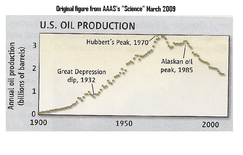
That brings up the question of oil supplies available. Here’s the US production history (actual data):

M. King Hubbert was the geologist who used an empirical curve fit to predict a US production peak in 1965 or 1970, back in 1956. His model takes advantage of a convenient mathematical curve shape, with no scientific causality built in, but was surprisingly accurate. He did this long before oil was discovered in Alaska. The effect of the new oil boom in "the Bakken" is another, larger hump (not shown) on the otherwise-decreasing overall trend. Its effects have temporarily reversed US production to a rise, but it is only temporary. The area under a Hubbert bell curve is proportional to the volume of the resource it models. Here is what that production history looks like with some Hubbert curves superimposed:

My conclusions follow:

---------------------------------------------------------
Update 6-5-2016: Later version of US production history from US EIA website, with Hubbert curve fit sketched upon it by me.

Note how different the fracking trend is, reflecting how fundamentally-different that recovery technology really is. Note also how the sharp rise suddenly cuts off right at the end of the data. The meaning of this is unclear at best. A logical question: how long will this boom last? Hubbert curves for smaller resource volumes tend to be narrower in time, looking "peaky".
------------------------------------------------------
In my opinion this makes (1) liars out of the US politicians running for office who told us we could drill our way out of dependence on foreign oil, and (2) fools out of those who believed them. The new oil boom has reversed this, but remember, that will be temporary!
The depletion of US oil reserves brings up the question of world oil depletion, and its effect on the basic supply-demand pricing level underneath the monopoly cartel pricing effects. The Saudis have not exceeded their own 2004 production levels. They sit on the 3 largest known remaining oil reserves left on the planet. It isn’t pretty:

But wait, some say we have tremendous reserves here at home. I see this claim quite a lot in email forwards about “the Bakken”, and some other names. These forwards always claim we have “cheap oil” in quantities exceeding Saudi Arabia, it’s just that the political opposition and/or environmentalists “won’t let us drill it”. These are just politically-motivated hit pieces. They mix facts with egregious lies and very slanted rhetoric. The truth is quite different. Bulletized list follows. I might add that the cleanup costs for the wastewater generated by the Alberta tar sands products we buy, are not in the product prices we pay, because they are as yet unknown. The volume of wastewater impounded under armed guard now exceeds Lake Erie. No one knows how to clean it up. That bill will come due. Soon.
Update: 3-5-13: Not long after I wrote this came word of a regional oil boom in the Williston Basin. They are using fracking in a thin dolomite layer sandwiched between Bakken shales to get a light crude. I documented this in a later article. Go see 9-5-11 "Surprise Surprise: Oil Boom in the Williston Basin (the "Bakken")". It's a small resource compared to the shales, which still refuse to yield oil.
Update 6-5-2016: the new fracking technology includes shale oil from "the Bakken", the south Texas oil shales, and more. See updated production history plot above.

So, as long as we use oil for fuel, we’re stuck with importing it. Most of those imports come from OPEC, dominated by middle eastern countries, some of whom are downright hostile. What do they do with all that money we have paid them for oil, for the past half century? You won’t like the answer:

We’ve been paying them to kill us. For decades. That does bring up good questions about treason.

There are a lot of entrenched interests long opposed to the implementation of alternative liquid transportation fuels, for a lot of “good-sounding” reasons. Yet there only three types of fuel to worry about, and three good drop-in alternatives available at one level or another, right now.

Gasoline can be stretched quite a bit further by blending-in significant ethanol, without any vehicle or infrastructure modifications (steel and neoprene are as good with ethanol as they are with gasoline). The only relevant questions are what source(s) do we use, and how much is available?

One of the specious arguments against ethanol is the effect of corn diversion from food use to fuel production. Many claim that the upsurge in food prices in 2009 was due to ethanol production. If you look at the actual facts, you find this claim is a lie.

To use ethanol successfully, we need the cellulosic technology that is just now being scaled-up and industrialized. This was originally made possible by grants from NREL, the alternative energy lab that has been part of DOE since Jimmy Carter’s time as president. Those first NREL grants made the industrial R&D possible, that in turn has recently led to pilot plant production of cellulosic ethanol at prices similar to gasoline, or cheaper. (That NREL/DOE story makes liars out of the authors of popular e-mail forwards claiming DOE has been a worthless waste, does it not?)
The situation is similar for using biodiesels in diesel fuel and jet fuel. The algae technology needs its development finished, so it can also be scaled up and industrialized. There’s more of it available.

OK, given that we finish the development, scale-up, and deployment of cellulosic ethanol and algae oils, what could we do with them? Remember, blend fuel products based on these materials are drop-in fuels, suitable even for the legacy fleets of old cars, old trucks, and old airplanes.
Answer: displace as much as possible of that imported oil we get from generally-hostile and financially-predatory OPEC. That picture still obtains, once the new oil boom fades.
If we go for E-33 and B-33 blend levels in the three fuels, this is what could happen:

The US could zero-out the imports it needs from OPEC! Wow!
If the US eliminates its dependence on OPEC oil, that is a major blow to the money OPEC funnels to the terrorists and proxy armies we fight, the US being their single largest customer by far. That has the added benefit of dropping oil prices via the supply-demand mechanism, compounding the denial of funds to the enemy. The rise of demand from rapidly-industrializing China and India has offset this; won't really happen.
If the rest of the western world followed suit, they and we together could dry up virtually all income to the Arab states of OPEC. Since those states have no other source of revenue (they have no other export the world wants), they would have to civilize themselves and join modern society as responsible members, or else go back to the stone age. And they know that (it is their greatest fear)! These nations can still be hurt if everybody just buys much less of their oil. Stretching fuel supplies with alternatives makes that happen, "Bakken" oil boom or not.
In other words, we could win this war economically, with no more invasions or armies. And, start making our economies proof against any more oil price-induced recessions, to boot.
The recent spate of low oil prices is only partially due to US fracking. The rest is mostly OPEC leaving their production rates high to deliberately force oil prices low. The motivation is two-fold: (1) trying to force US frackers out of the business with prices too low to support that activity, and (2) fear of losing market share as an individual country, if any of them do cut back.
I was surprised and pleased to learn that there really was shale oil producible by fracking. What they appear to be recovering is a "light sweet crude" that actually resembles diesel fuel in its physical properties. This is unlike most crudes, which are much thicker and less mobile, and far less volatile. That volatility is the source of the dangers experienced while shipping this stuff by rail, because there aren't enough of the safer pipelines.
The shales in south Texas are producing this kind of crude, and also the Williston basin formations, most notably in Wyoming. I have seen no figures on what percentage of the hydrocarbons in the rock pores are being recovered, but I'd still bet it's single digit, or not much better. It's just a rich enough set of resources to make recovery feasible, as long as prices are not too low.
The fundamental side effect we are incurring is used frack water. It comes back as a concentrated brine contaminated with heavy metals, other mineral poisons (like arsenic), leftover cancer-causing hydrocarbons (like benzene) from the frack fluid additives, and radioactivity leached from the deep rocks.
No one is re-using this fluid, and there is really not enough fresh water around to fill the demand. Plus, deep well injection disposal is causing earthquakes in north Texas and in Oklahoma, at least. Long term, the solution is obviously re-using frack water (reducing demand on limited supplies of fresh water, and greatly reducing the disposal quantities). That will require developing an additive package that works in brine (which makes sea water feasible as a feedstock source). I can think of nothing that should not be higher on DOE's R&D list.
There are still strong conflicts over whether fracking pollutes ground water. My hunch is that they'd better look closer at the geology in which they frack, and also at well casing quality. Eliminate cheap leaky well casings, and the only other way for natural gas to surface (besides the well) is directly through the rocks. Rock layers that are relatively unfolded and unbroken won't leak very badly. Fractured, folded rocks in mountainous zones will leak very badly. It may well be that simple.
--- GW
Update 1-3-15 at bottom in black.
Updates 2-4-14 below in blue.
Update 6-5-2016 in purple:
I went and looked up a US oil production history curve similar to the one I saw from the 2009 "Science" article used in the article below. I inserted it below adjacent to the older plot for easy comparison. With another 5 years' of history, it is pretty easy to see the Hubbert curve shape in the conventional oil recovery history of US production up to about 2011, and that the Alaska "bump" is actually a fairly small effect.
The fracking technology is a larger effect than I believed at the time. It is a fundamentally new and different production technology, which makes both new shale resources available, and more recovery feasible from older depleted fields. This is a very steep rise ion production, with very little time history yet to interpret trends. It is premature to judge yet, but the steep rise does suggest the narrower Hubbert curve shape of a smaller volume to be recovered.
The Saudis more-or-less lead OPEC in production quotas and prices, but are adversarial with Iran, who is reentering the mass market. All the OPEC countries are afraid of losing market share if they cut back, but are being hurt by lower prices. Yet if they continue to hold prices down by over-production, they may cut off the US fracking boom, which is a fundamentally more expensive technique. We'll see, but the verdict won't come for some years yet.
----------------------------------------------------------------------------------------------------------
By putting together facts from different sources, adding in some events from recent history, and a little common sense, one can draw some startling conclusions. These should make you as mad as they do me. It’s hard to argue with factual data. My conclusions are my own opinions. You draw conclusions for yourself, and form your own opinions.
I start with a graph of US regular gasoline price history from about 1970 to the present, adjusted for inflation, as January 2011-dollar equivalent. I got this from “zfacts.com”, which has quite the variety of both facts and opinions. Price history is fact, not opinion, however.

To this time history graph, I added several historical events, a line representing the current equivalent of 1958’s 25 cent/gallon gasoline, and a second line representing a conclusion I drew from all this data regarding recessions. That modified chart is complicated and takes a while to digest, but here it is:

I was able to discern several connections between this price history and contemporary events, as well as linkages between fuel prices and recessionary events. These are listed in bullet form on the next graphic. The most important one is in capital letters. It makes liars out of most US politicians running for office, from either party. The notion of an enormous monopoly-cartel pricing effect superposed on top of a basic supply-demand price level, makes liars out of those who claim the international oil market is nothing but a “free market”, for it most clearly is not. There is also a price speculation effect superposed on top of supply-and-demand effects. The scariest bullet is the very last one, however.

That brings up the question of oil supplies available. Here’s the US production history (actual data):
M. King Hubbert was the geologist who used an empirical curve fit to predict a US production peak in 1965 or 1970, back in 1956. His model takes advantage of a convenient mathematical curve shape, with no scientific causality built in, but was surprisingly accurate. He did this long before oil was discovered in Alaska. The effect of the new oil boom in "the Bakken" is another, larger hump (not shown) on the otherwise-decreasing overall trend. Its effects have temporarily reversed US production to a rise, but it is only temporary. The area under a Hubbert bell curve is proportional to the volume of the resource it models. Here is what that production history looks like with some Hubbert curves superimposed:

My conclusions follow:

---------------------------------------------------------
Update 6-5-2016: Later version of US production history from US EIA website, with Hubbert curve fit sketched upon it by me.

Note how different the fracking trend is, reflecting how fundamentally-different that recovery technology really is. Note also how the sharp rise suddenly cuts off right at the end of the data. The meaning of this is unclear at best. A logical question: how long will this boom last? Hubbert curves for smaller resource volumes tend to be narrower in time, looking "peaky".
------------------------------------------------------
In my opinion this makes (1) liars out of the US politicians running for office who told us we could drill our way out of dependence on foreign oil, and (2) fools out of those who believed them. The new oil boom has reversed this, but remember, that will be temporary!
The depletion of US oil reserves brings up the question of world oil depletion, and its effect on the basic supply-demand pricing level underneath the monopoly cartel pricing effects. The Saudis have not exceeded their own 2004 production levels. They sit on the 3 largest known remaining oil reserves left on the planet. It isn’t pretty:

But wait, some say we have tremendous reserves here at home. I see this claim quite a lot in email forwards about “the Bakken”, and some other names. These forwards always claim we have “cheap oil” in quantities exceeding Saudi Arabia, it’s just that the political opposition and/or environmentalists “won’t let us drill it”. These are just politically-motivated hit pieces. They mix facts with egregious lies and very slanted rhetoric. The truth is quite different. Bulletized list follows. I might add that the cleanup costs for the wastewater generated by the Alberta tar sands products we buy, are not in the product prices we pay, because they are as yet unknown. The volume of wastewater impounded under armed guard now exceeds Lake Erie. No one knows how to clean it up. That bill will come due. Soon.
Update: 3-5-13: Not long after I wrote this came word of a regional oil boom in the Williston Basin. They are using fracking in a thin dolomite layer sandwiched between Bakken shales to get a light crude. I documented this in a later article. Go see 9-5-11 "Surprise Surprise: Oil Boom in the Williston Basin (the "Bakken")". It's a small resource compared to the shales, which still refuse to yield oil.
Update 6-5-2016: the new fracking technology includes shale oil from "the Bakken", the south Texas oil shales, and more. See updated production history plot above.

So, as long as we use oil for fuel, we’re stuck with importing it. Most of those imports come from OPEC, dominated by middle eastern countries, some of whom are downright hostile. What do they do with all that money we have paid them for oil, for the past half century? You won’t like the answer:

We’ve been paying them to kill us. For decades. That does bring up good questions about treason.

There are a lot of entrenched interests long opposed to the implementation of alternative liquid transportation fuels, for a lot of “good-sounding” reasons. Yet there only three types of fuel to worry about, and three good drop-in alternatives available at one level or another, right now.

Gasoline can be stretched quite a bit further by blending-in significant ethanol, without any vehicle or infrastructure modifications (steel and neoprene are as good with ethanol as they are with gasoline). The only relevant questions are what source(s) do we use, and how much is available?

One of the specious arguments against ethanol is the effect of corn diversion from food use to fuel production. Many claim that the upsurge in food prices in 2009 was due to ethanol production. If you look at the actual facts, you find this claim is a lie.

To use ethanol successfully, we need the cellulosic technology that is just now being scaled-up and industrialized. This was originally made possible by grants from NREL, the alternative energy lab that has been part of DOE since Jimmy Carter’s time as president. Those first NREL grants made the industrial R&D possible, that in turn has recently led to pilot plant production of cellulosic ethanol at prices similar to gasoline, or cheaper. (That NREL/DOE story makes liars out of the authors of popular e-mail forwards claiming DOE has been a worthless waste, does it not?)
The situation is similar for using biodiesels in diesel fuel and jet fuel. The algae technology needs its development finished, so it can also be scaled up and industrialized. There’s more of it available.

OK, given that we finish the development, scale-up, and deployment of cellulosic ethanol and algae oils, what could we do with them? Remember, blend fuel products based on these materials are drop-in fuels, suitable even for the legacy fleets of old cars, old trucks, and old airplanes.
Answer: displace as much as possible of that imported oil we get from generally-hostile and financially-predatory OPEC. That picture still obtains, once the new oil boom fades.
If we go for E-33 and B-33 blend levels in the three fuels, this is what could happen:

The US could zero-out the imports it needs from OPEC! Wow!
If the US eliminates its dependence on OPEC oil, that is a major blow to the money OPEC funnels to the terrorists and proxy armies we fight, the US being their single largest customer by far. That has the added benefit of dropping oil prices via the supply-demand mechanism, compounding the denial of funds to the enemy. The rise of demand from rapidly-industrializing China and India has offset this; won't really happen.
If the rest of the western world followed suit, they and we together could dry up virtually all income to the Arab states of OPEC. Since those states have no other source of revenue (they have no other export the world wants), they would have to civilize themselves and join modern society as responsible members, or else go back to the stone age. And they know that (it is their greatest fear)! These nations can still be hurt if everybody just buys much less of their oil. Stretching fuel supplies with alternatives makes that happen, "Bakken" oil boom or not.
In other words, we could win this war economically, with no more invasions or armies. And, start making our economies proof against any more oil price-induced recessions, to boot.
Update 1-3-15:
The recent explosion of US “fracking” technology (hydraulic
fracturing plus horizontal-turn drilling) has modified the picture of oil
prices versus recessions.
Unexpectedly, the US has become a
leading producer of crude oils for the world market. Plus,
there has been an associated massive production increase and price drop
in natural gas.
OPEC has chosen to take the income “hit” and not cut back
their production in response. Their
reasoning is twofold: (1) fear of loss
of market share, and (2) hope that low
oil prices will curtail US “fracking” recoveries. We will see how that plays-out.
Oil prices are now such (at around $55/barrel) that US
regular gasoline prices are nearing $2.00/gal for the first time in a very long
time. This is very close to the price
one would expect for a truly competitive commodity, based on 1958 gasoline prices in the US, and the inflation factor since then.
It is no coincidence that the exceedingly-weak US “Great Recession”
recovery has suddenly picked up steam.
The timing of the acceleration in our economic recovery versus the
precipitous drop in oil prices is quite damning. There can be no doubt that
higher-than-competitive-commodity oil prices damage economies. Oil prices are a superposition of the competitive
commodity price, overlain by an erratic
increase from speculation, and further overlain
quite often by punitive price levels when OPEC is politically unhappy with the
west. That’s been the history.
This economic improvement we are experiencing will persist
as long as oil, gas, and fuel prices remain low. (Government policies have almost nothing to
do with this, from either party.) How long that improvement continues depends
in part upon US “fracking” and in part upon OPEC. Continued US “fracking” in the short term may
depend upon adequate prices. In the long
term, we need some solutions to some
rather intractable problems to continue our big-time “fracking” activities.
The long-term problems with “fracking” have to do with (1)
contamination of groundwater with combustible natural gas, (2) induced earthquake activity, (3) lack of suitable freshwater supply to
support the demand for “fracking”, and
(4) safety problems with the transport of the volatile crude that “fracking”
inherently produces.
Groundwater
Contamination
Groundwater contamination is geology-dependent. In Texas,
the rock layers lie relatively flat,
and are relatively undistorted and unfractured. This is because the rocks are largely old sea
bottom that was never subjected to mountain-building. We Texans haven’t seen any significant
contamination of ground water by methane freed from shale. The exceptions trace to improperly-built
wells whose casings leak.
This isn’t true in the shales being tapped in the
Appalachians, or in the shales being
tapped in the eastern Rockies. There the
freed gas has multiple paths to reach the surface besides the well, no matter how well-built it might have
been. Those paths are the vast
multitudes of fractures in the highly-contorted rocks that subject to mountain-building
in eons past. That mountain-building may
have ceased long ago, but those cracks
last forever.
This is why there are persistent reports of kitchen water
taps bursting into flames or exploding,
from those very same regions of the country. It’s very unwise to “frack” for gas in that
kind of geology.
Induced Earthquake
Activity
This does not seem to trace to the original “fracking”
activity. Instead it traces rather
reliably to massive injections of “fracking” wastewater down disposal
wells. Wherever the injection quantities
are large in a given well, the frequent
earthquakes cluster in that same region.
Most are pretty weak, under
Richter magnitude 3, some have
approached magnitude 4.
There is nothing in our experience to suggest that magnitude
4 is the maximum we will see. No
one can rule out large quakes. The risk is with us as long as there are
massive amounts of “fracking” wastewater to dispose of, in these wells. As long as we never re-use “frack”
water, we will have this massive
disposal problem, and it will induce
earthquakes.
Lack of Freshwater
Supply to Support “Fracking”
It takes immense amounts of fresh water to “frack” a single
well. None of this is ever re-used, nor it is technologically-possible to
decontaminate water used in that way. The
additives vary from company to company,
but all use either sand or glass beads,
and usually a little diesel fuel.
Used “frack” water comes back at near 10 times the salinity of sea
water, and is contaminated by heavy
metals, and by radioactive minerals, in addition to the additives. Only the sand or glass beads get left
behind: they hold the newly-fractured
cracks in the rocks open, so that
natural gas and volatile crudes can percolate out.
The problem is lack of enough freshwater supplies. In most areas of interest, there is not enough fresh water available to
support both people and “fracking”, especially
with the drought in recent years. This assessment
completely excludes the demand increases due to population growth. That’s even worse.
This problem will persist as long as fresh water is used for
“fracking”, and will be much, much worse as long as “frack” water is not
reused. The solution is to start with
sea water, not fresh water, and then to re-use it. This will require some R&D to develop a
new additive package that works in salty water to carry sand or glass
beads, even in brines 10 times more
salty than sea water.
Nobody wants to pay for that R&D.
Transport Safety with
Volatile “Frack” Crudes
What “fracking” frees best from shales is natural gas, which is inherently very mobile. Some shales (by no means all of them) contain
condensed-phase hydrocarbons volatile enough to percolate out after hydraulic
fracturing, albeit more slowly than
natural gas. Typically, these resemble a light, runny winter diesel fuel, or even a kerosene, in physical properties. More commonly, shale contains very immobile condensed
hydrocarbons resembling tar. These cannot
be recovered by “fracking” at all.
The shales in south Texas,
and some of the shales and adjacent dolomites in the Wyoming region
actually do yield light, volatile
crudes. The problem is what to transport
them in. There are not enough
pipelines to do that job. Pipelines are safer
than rail transport, all the spills and
fires notwithstanding.
The problem is that we are transporting these
relatively-volatile materials in rail tank cars intended for normal (heavy)
crude oils, specifically DOT 111 tank cars. Normal crudes are relatively-nonvolatile and
rather hard to ignite in accidents. DOT
111 cars puncture or leak frequently in derail accidents, but this isn’t that serious a problem as long
as the contents are non-volatile. These
shale-“frack” light crude materials resemble nothing so much as No. 1 winter
diesel, which is illegal to ship in DOT
111 cars, precisely since it is too
volatile.
The problem is that no one wants to pay for expanding the
fleet of tougher-rated tank cars. So, many outfits routinely mis-classify “frack” light
crudes as non-volatile crudes, in order
to “legally” use the abundant but inadequate DOT-111 cars. We’ve already seen the result of this kind of
bottom line-only thinking, in a series
of rather serious rail fire-and-explosion disasters, the most deadly (so far) in Lac
Megantic, Quebec.
Volatile shale-“fracked” crudes simply should not be shipped
in vulnerable DOT 111 cars, period. It is demonstrably too dangerous.
Conclusions
“Fracking” shales for natural gas and light crudes has had a
very beneficial effect on the US economy and its export-import picture. We should continue this activity as a
reliable bridge to things in the near future that are even better.
But, we must address
the four problem areas I just outlined.
And I also just told you what the solutions are. The problem is, as always,
who pays. What is the value of a
human life? What is the value of a
livable environment? It’s not an either-or
decision, it’s striking the appropriate balance!
Thursday, February 3, 2011
How to Drive on Icy Roads
Roads tend to get beaten "clean" in ruts, especially in the southlands. Drive in those ruts, there's better traction there. Just slow down until you feel no hint of fishtail instability, and then another 5 or 10 mph slower. It's that simple.
Your enemy is bridges and big culverts. These tend to accumulate more and slicker ice, and they ice-up first. The sand (if any) helps only for a little while, then the wetted sand and slush re-freezes into a new and harder coating that is just as slick as plain ice, and a whole lot harder to pound loose by the passage of traffic. Never, ever assume a bridge is safe! Turn your flasher on to warn the folks behind you, that you are doing something they don't expect, and slow way down before you reach the bridge. Most cars have a maximum controllable speed on slick ice in the neighborhood of 20 mph. You need to be moving at least that slow as you reach the bridge, so you can see what's really on it, in time to respond. Plain and simple.
If the bridge has clean ruts or is clean and dry, speed back up and cross. Stay within the ruts. If the bridge is icy, stay under that 20 mph. Steer to cross the bridge in a straight line, get off the gas and brake (and stay off them) and make no steering changes while you coast across. You will come out just fine on the other side, if you do these things. You will not come out fine, if you accelerate, brake, or turn, in the slightest. For long bridges, modify this as absolutely-constant speed driving, no braking, no turning, at substantially less than 20 mph. I recommend about 10-15 mph for most cars.
For roads with paved shoulders, there is usually gravel on the shoulder and a few inches beyond. If you start fishtailing before you can slow, put two wheels into that grass and gravel right at the edge of the shoulder. Your fishtailing will stop. But, don't stay there, decelerate by coasting, and put it back onto the road, before you get stuck. Don't do this on a farm-to-market road, there are no shoulders, and the ground off the pavement is generally too soft (because of the precipitation). Just drive much slower on those roads, so that you never fishtail.
Pickup trucks and front-engine, rear-drive cars are extremely prone to rear-end-breakaway skids, because the weight distribution is very bad for all-wheel traction. You need to go much slower than a ordinary car, because once it breaks away, you are out of control, and you won't get it back until you come pretty much to rest (which might entail fetching up against something really solid). It'll warn you by feeling very unsteady, by wanting to fishtail. Find the fishtail speed for your vehicle (not in traffic, please!), and then drop at least 10 mph below that. Be aware that this speed changes as conditions change.
SUV's are famous for being able to "go" when other vehicles won't, especially the 4-wheel-drive ones. But, they do not stop any better than the worst of the conventional cars, and they are far more unstable due to the high center of gravity. I've seen more SUV's upside down in medians and bar ditches, than any other type of vehicle. Slow way down!
The vehicles with more even weight distributions front-to-back can suffer from the other type of skid: front end breakaway. That's when you crank the steering wheel to turn and nothing happens. Why? You are going too fast. Steer straight and miss the turn, coast down, and drive a lot slower. The problem will go away if you slow down. If this happens on a curve, the only thing you can try is a shallower turn. Do not brake (you will spin out), do not accelerate (same result). Very gentle steering inputs will sometimes work when a big input fails. Trouble is, most of the time, you don't have room for that. So, I recommend you try your vehicle out turning on the ice in an empty parking lot. Look for the speed at which it breaks away, and back off at least 10 mph below that. Use that reduced speed figure as your maneuvering speed out there on the icy road.
Some folks put chains on. They work, but rarely are they rated for driving more than 10 or 15 mph. You can pretty much do just as well without them, at those low speeds. Drive too fast, and they come apart. The flying fragments are steel shrapnel. They will damage your car, and they will hurt innocent bystanders. I haven't owned chains in decades. No need.
Don't forget to turn on your lights. This is as much to be seen by others, as it is for you to see better. In the fog, mist, and snow, all colors are "stealth", even reds and yellows.
And don't forget to wear your seat belts. If you don't know what you're doing, or have little practice, driving on ice, chances are actually very high you will have at least a minor accident. Could easily be a major accident. Belts make the difference between a bruised ego and a hospital stay. Or death.
If you get stuck, and you can almost but not quite "rock" your way out using forward and reverse, then try using the vehicle's floor mats. Put one, textured rubber side up, under each drive wheel. For marginal cases, that's often just enough extra traction to get free. Better to get tire tread marks and dirt on your mats, than to freeze while waiting for rescue.
Finally, dress for it! Dress like you have to walk miles in the snow and wind and cold. You very well might have to.
Your enemy is bridges and big culverts. These tend to accumulate more and slicker ice, and they ice-up first. The sand (if any) helps only for a little while, then the wetted sand and slush re-freezes into a new and harder coating that is just as slick as plain ice, and a whole lot harder to pound loose by the passage of traffic. Never, ever assume a bridge is safe! Turn your flasher on to warn the folks behind you, that you are doing something they don't expect, and slow way down before you reach the bridge. Most cars have a maximum controllable speed on slick ice in the neighborhood of 20 mph. You need to be moving at least that slow as you reach the bridge, so you can see what's really on it, in time to respond. Plain and simple.
If the bridge has clean ruts or is clean and dry, speed back up and cross. Stay within the ruts. If the bridge is icy, stay under that 20 mph. Steer to cross the bridge in a straight line, get off the gas and brake (and stay off them) and make no steering changes while you coast across. You will come out just fine on the other side, if you do these things. You will not come out fine, if you accelerate, brake, or turn, in the slightest. For long bridges, modify this as absolutely-constant speed driving, no braking, no turning, at substantially less than 20 mph. I recommend about 10-15 mph for most cars.
For roads with paved shoulders, there is usually gravel on the shoulder and a few inches beyond. If you start fishtailing before you can slow, put two wheels into that grass and gravel right at the edge of the shoulder. Your fishtailing will stop. But, don't stay there, decelerate by coasting, and put it back onto the road, before you get stuck. Don't do this on a farm-to-market road, there are no shoulders, and the ground off the pavement is generally too soft (because of the precipitation). Just drive much slower on those roads, so that you never fishtail.
Pickup trucks and front-engine, rear-drive cars are extremely prone to rear-end-breakaway skids, because the weight distribution is very bad for all-wheel traction. You need to go much slower than a ordinary car, because once it breaks away, you are out of control, and you won't get it back until you come pretty much to rest (which might entail fetching up against something really solid). It'll warn you by feeling very unsteady, by wanting to fishtail. Find the fishtail speed for your vehicle (not in traffic, please!), and then drop at least 10 mph below that. Be aware that this speed changes as conditions change.
SUV's are famous for being able to "go" when other vehicles won't, especially the 4-wheel-drive ones. But, they do not stop any better than the worst of the conventional cars, and they are far more unstable due to the high center of gravity. I've seen more SUV's upside down in medians and bar ditches, than any other type of vehicle. Slow way down!
The vehicles with more even weight distributions front-to-back can suffer from the other type of skid: front end breakaway. That's when you crank the steering wheel to turn and nothing happens. Why? You are going too fast. Steer straight and miss the turn, coast down, and drive a lot slower. The problem will go away if you slow down. If this happens on a curve, the only thing you can try is a shallower turn. Do not brake (you will spin out), do not accelerate (same result). Very gentle steering inputs will sometimes work when a big input fails. Trouble is, most of the time, you don't have room for that. So, I recommend you try your vehicle out turning on the ice in an empty parking lot. Look for the speed at which it breaks away, and back off at least 10 mph below that. Use that reduced speed figure as your maneuvering speed out there on the icy road.
Some folks put chains on. They work, but rarely are they rated for driving more than 10 or 15 mph. You can pretty much do just as well without them, at those low speeds. Drive too fast, and they come apart. The flying fragments are steel shrapnel. They will damage your car, and they will hurt innocent bystanders. I haven't owned chains in decades. No need.
Don't forget to turn on your lights. This is as much to be seen by others, as it is for you to see better. In the fog, mist, and snow, all colors are "stealth", even reds and yellows.
And don't forget to wear your seat belts. If you don't know what you're doing, or have little practice, driving on ice, chances are actually very high you will have at least a minor accident. Could easily be a major accident. Belts make the difference between a bruised ego and a hospital stay. Or death.
If you get stuck, and you can almost but not quite "rock" your way out using forward and reverse, then try using the vehicle's floor mats. Put one, textured rubber side up, under each drive wheel. For marginal cases, that's often just enough extra traction to get free. Better to get tire tread marks and dirt on your mats, than to freeze while waiting for rescue.
Finally, dress for it! Dress like you have to walk miles in the snow and wind and cold. You very well might have to.
Friday, January 21, 2011
Fundamental Design Criteria for Alternative Space Suit Approaches
This posting supports the manned Mars mission design posting of 7-25-11. The supple space suit discussed here is presumed to exist for that mission.
Update 10-11-13: See also 4-17-10 "Space Recommendations".
The focus here is the so-called mechanical counterpressure (MCP) space suit. This was a design approach explored (among other things) on the PBS program “Nova Science Now”, aired Wednesday, January 19, 2011, in Texas. This approach has its genesis in the “partial pressure suits” used by USAF in the late 1940’s, and during the 1950’s. It was tested as a possible space suit design with the elastic fabrics of the 1960’s, and in the last decade has come back under consideration again, as a possible way to vastly improve astronaut mobility and dexterity.
General Considerations:
Here on Earth, our atmosphere contains the oxygen we need to support life, and it also exerts its pressure upon our bodies. This pressure has two effects: (1) to concentrate the oxygen enough to diffuse effectively into our blood across the alveoli structures in our lungs, and (2) to keep the water in our blood and tissues from boiling away at body temperature. The minimum partial pressure of oxygen necessary for effective respiration is an indistinct limit, but it is substantially higher than the value of external pressure necessary to keep our blood and tissue moisture from boiling away. This boil-off level is pretty close to the equilibrium vapor pressure of water at a body temperature of 98.6 F (37.0 C), which is 0.06192 of a standard atmosphere.
In space, there is no oxygen and there is no pressure. Unprotected persons die quickly, first losing consciousness in seconds to a couple of minutes, due to anoxia, then suffering anoxic brain death within a very few more minutes (around 10), which event is generally irreversible. Some several minutes after the onset of brain death, the heart stops and blood pressure falls below the moisture boil-off level. The water in the blood and tissues begins to boil away into space, breaking open cell membranes and splitting open tissue structures. Boil-off of this moisture draws heat from the surrounding tissue structures, chilling the body rapidly toward freezing as it partially desiccates.
Thus, a protective enclosure is necessary for us to survive in space, one which provides oxygen at a suitable pressure inside the lungs and breathing passages. This breathing gas pressure must be balanced by the same fluid pressure within the body, in turn produced by an equal pressure applied to the external surface of the body. An important fact: this external pressure can be supplied in two ways: (1) by gas or fluid pressure within a sealed garment that is essentially a balloon, or (2) mechanical pressure applied directly to (and distributed over) the skin.
Historical Specifics:
By about 1930, high-flying pilots had to be protected from lack of oxygen. One way was a modified deep-sea diver’s dress, functioning as a pressurized balloon. The atmosphere inside the sealed garment could be pure oxygen instead of air, and its pressure need only be enough to concentrate the oxygen in the lungs sufficient to support respiration. Such pressures are typically well above the moisture boil-off level. This balance of breathing gas vs internal tissue fluid pressures, with a distributed external pressure creating those internal fluid pressures, is illustrated in the right hand portion of figure 1. The creation of those internal tissue fluid pressures is very much like squeezing a water balloon all over, raising its internal pressure, as in the center portion. This works because the cells of the body are essentially tiny water balloons. Thus, in the aggregate, the body responds like the water balloon.

Figure 1 – Pressure Balance Physics with Fluid-Filled Objects and Aggregates of Same
Military pilots flying “high-gee” maneuvers tend to faint, because the blood supplying oxygen to their brains is pulled by the high accelerations toward their lower extremities (pooling in their legs). Hypoxia thus induced soon leads to blackout, often within a very few seconds. The solution is to drive that blood supply upward against the acceleration by means of the “gee suit”. These garments provide a mechanical squeezing action on the lower body and legs, similar to squeezing just part of a water balloon. This uneven compression drives the fluid within toward the uncompressed portion, instead of generally increased internal pressure. This action is illustrated in the left portion of figure 1. In the water balloon, the unsqueezed portion expands with the extra water driven there. In the body, blood that would have pooled in the legs is driven upward against the acceleration back to the brain.
In the late 1940’s, this “gee-suit” action was proposed as a temporary protection garment for test and fighter pilots having to bail out or deal with loss of cabin pressure at extreme altitudes. By this time, it was already known that an ordinary oxygen mask could not supply a sufficient concentration of oxygen, because the atmospheric external pressure governing that concentration was too low. (The critical altitude for that is a little “fuzzy”, but generally we use 45,000 feet.) Pressure breathing gear was required for flying higher, and this required a counterbalancing internal tissue fluid pressure within the body (as illustrated in the right-hand portion of figure 1). The balloon-type pressure suits of that time were simply too restrictive of movement, too bulky, and too heavy, to serve in this application.
An extension of the gee suit mechanical compression approach provided the answer used in the late 1940’s and 1950’s: the so-called “partial pressure suit”. The mechanical compression was extended over most of the body, providing internal fluid pressures more or less sufficient to balance breathing gas pressures in a helmet, in turn adequate to support life long enough to bail out from around 100,000-foot altitudes. It wasn’t perfect: hands and feet remained uncompressed, and the actual compression achieved over the torso and limbs was very uneven. Blood pooling within inadequately compressed limbs would lead to the pilot blacking out, in about 10 minutes or so, and serious swelling from edema within about an hour. But, it worked well enough to serve for the few minutes of a bailout or emergency descent. Compression was achieved by tensioning the non-elastic fabric across the skin by inflatable “capstans” (tubes). These suits were far less restrictive of movement, far less bulky, and far lighter than the gas balloon-type pressure suits of that time.
By the end of the 1950’s, the gas balloon suits had been sufficiently improved to be competitive with the partial pressure suit in terms of bulk, weight, and movement restrictions. These newer gas balloon suits (“full pressure suits”) had no restriction on protection time, as an even distribution of compression was inherently achieved on all body parts. This eliminates blood pooling problems. Thus, these were chosen as the space suits of the 1960’s, and have been the standard ever since. As evolved for in-space and lunar use since then, these have become very bulky, restrictive garments. Cooling systems are required inside the hermetically-sealed suit. Due to the stiffness and bulk of the pressurized gloves, manual dexterity is very limited. Typically, the suit pressure used is 1/3 of an atmosphere of pure oxygen, near 253 mm Hg.
In the late 1960’s, the partial pressure suit problems of uneven compression distributions and limited coverage were addressed fairly successfully by the use of elastic fabrics. By mechanically compressing the hands and feet as well as the limbs and torso, time-unlimited protection could be had. Such garments need not be one piece, as they were not gas-tight balloons, merely the equivalent of tight panty hose or shrink-wrap. Tailoring the distribution and arrangement of layers of elastic fabric in the various garment sections was the hard part. No cooling system was required: the wearer could sweat right through the porous garment into vacuum. Such a space suit was demonstrated as a prototype in the vacuum tank successfully, under the direction of Dr. Paul Webb, and partly funded by NASA. Including the oxygen supply and helmet, it weighed 85 pounds, with little movement restriction, and marvelous dexterity. Compare that with the 200+ pound full pressure suits used on the moon! The breathing pressure was in the neighborhood of 170-190 mm Hg. These efforts did not lead to application then.
The mechanical compression idea has resurfaced in the last decade, including efforts for NASA. The modern ability to tailor elastic fabrics is even better than that available in the late 1960’s. Up to a certain level of mechanical compression, these techniques now work fine. The level currently achievable is not 1/3 of an atmosphere, however. But, is that level really necessary, considering that the experiments of the late 1960’s were successful with much lower compression? This is important, because if one specifies a compression level higher than can be reached with the technology, this MCP technique could be deemed infeasible, when in fact it is feasible, and offers some very significant advantages.
Design Criteria for Breathing Pressures:
A good startpoint is the concentration of oxygen available to people at sea level. The standard oxygen content of dry air is generally thought to be 20.946 volume percent (v%). One standard atmosphere’s pressure is defined as 14.696 psia, 1013.25 mbar, 29.92 inch Hg (mercury manometer column height), or 760 mm Hg. The gas laws indicate that partial pressure percentages are the same as volume percent composition. See figure 2. At sea level, the partial pressure of oxygen in dry air is then 159.2 mm Hg.
Inside the moist lungs the air is no longer dry. A fairly realistic assumption is that the water vapor is saturated. Water vapor pressure is determined at equilibrium by the temperature of the liquid phase in contact with it, in this case, body temperature of a human (98.6 F or 37.0 C). From the standard steam tables, this vapor pressure is 47.1 mm Hg. That vapor displaces some of the dry air, so that the partial pressures of the dry air and the water vapor now add to the imposed atmospheric pressure, in this case sea level (760 mm Hg). The oxygen partial pressure in the wetted air freshly inhaled into the lungs is then 20.946% of the dry air partial pressure (712.9 mm Hg), or about 149.3 in Hg.
Between inhale and exhale, some of this oxygen is diffused across the alveoli into the blood, and some carbon dioxide diffuses from the blood back into the air in the lungs. Compared to the water vapor displacement effect, these transient effects are small, and are ignored here.
What drives diffusion of oxygen into the blood is the partial pressure of oxygen in the wet air inside the lungs. This must be larger than the dissolved oxygen pressure in the blood for diffusion to occur at a useful rate. Therefore, there is a lower limit to the in-lung partial pressure of oxygen, but it is a little “fuzzy”, and must be determined empirically. The calculation of in-lung oxygen concentrations from atmospheric air at altitude pressure, and their relationship to pure oxygen breathing pressures in a suit, is illustrated in figure 2. It should be noted that the water vapor pressure is a constant set by body temperature, having a larger percentage effect at high-altitude lower atmosphere pressures, and at lower suit oxygen pressures.

Figure 2 – In-Lung Oxygen Estimates from Air at Altitude and In-Suit Oxygen
One estimate of the lower limit for in-lung oxygen concentration comes from in-flight oxygen rules for pilots. Civilian pilots are not required to use oxygen below 10,000 feet altitude under US FAA rules (the USN uses a different figure: 5000 feet). Most other agencies use something like the 10,000 foot rule. Using the procedure outlined in figure 2 at sea level and at 10,000 feet atmosphere pressures produces the results bordered in green in figure 3. For people adapted to more-or-less sea level air, in-lung oxygen partial pressures in the range 149.3 down to 99.6 mm Hg seem quite adequate. These correspond to altitudes in air from sea level up to 10,000 feet. They also correspond to oxygen breathing gas and suit compression pressure levels of 196.4 down to 146.7 mm Hg. These are 25.8 down to 19.3% of a standard atmosphere as the suit compression levels required.
Using the current full pressure suit standard of 1/3 atmosphere pure oxygen (253.3 mm Hg), one has a wet in-lung oxygen of partial pressure of 206.3 mm Hg, substantially more than in sea level air. These are the data bordered in blue in figure 3. They do not correspond to a calculated altitude, which would be far below sea level. Clearly, 33% of a standard atmosphere is an over-stringent pressurization requirement for the MCP suit. Something closer to 25% of an atmosphere is equivalent to sea level air, and serves well as an upper limit for MCP compression design.

Figure 3 – Suit Compression Levels Corresponding to In-Lung Oxygen at Various Altitudes
There are populations of humans who live at very high altitudes. Substantial numbers of people live near 15,000 feet , corresponding to in-lung oxygen near 80 mm Hg, and further corresponding to a suit compression level of 127 mm Hg (16.7% of an atmosphere). However these people are acclimatized to these conditions. It takes substantial time for the body to so acclimatize. Without that acclimatization, altitude sickness and fainting are high risks. There are a few people living near 20,000 feet in the high Andes or Himalayas. That altitude corresponds to in-lung oxygen 63.4 mm Hg, and suit compression 110 mm Hg (14.5% of an atmosphere). The 15,000 and 20,000 foot calculated data are included in the figure 3 table bordered yellow. “Flatlanders” in space suits at those pressures would survive, but would not be functional. Therefore, the 10,000 foot data make a pretty good empirical lower limit for MCP suit compression design.
Further, consider the nominal 45,000 foot requirement for something better than a simple oxygen mask. Those data are included as one of two entries in the red-bordered portion of figure 3. At that altitude with pure oxygen in a simple mask, in-lung oxygen is 64 mm Hg, and external compression is 111 mm Hg (14.6% of an atmosphere). Those levels correspond very closely with the in-lung oxygen levels of long-acclimatized mountain folks living in the open air near 20,000 feet. That is a good rough estimate of an extreme lower compression limit to stave off certain slow death by hypoxia.
The other entry in the red-bordered portion of figure 3 is the moisture boil-off point (where the blood starts to boil, and tissues outgas water vapor as they begin to desiccate and freeze). There is no oxygen at all in the lungs at this pressure; it is all water vapor at 47 mm Hg, which has to be the external compression pressure. Those figures correspond to 64,000 feet altitude and 6.2% of an atmosphere. About 60,000 feet has long been thought to be the short-exposure “deathpoint” for risk of blood boiling.
Conclusions:
The minimum design compression for an MCP-type space suit is very likely near 19 or 20% of a standard atmosphere (147 mm Hg), corresponding very closely with the in-lung wet oxygen partial pressure of 99.6 mm Hg experienced in the open air at 10,000 feet. Compressing less risks dysfunction.
The maximum necessary design compression for an MCP-type space suit is near 25 or 26% of a standard atmosphere (196 mm Hg), corresponding very closely with the in-lung wet oxygen partial pressure of 149 mm Hg experienced in the open air at sea level. It does not hurt to compress more.
The “typical” space suit design standard of 33% of an atmosphere seems to be an unnecessarily stringent design requirement, especially if fabric technology cannot quite achieve it right now.
Related Articles on this Site:
Update 10-11-13: See also 4-17-10 "Space Recommendations".
The focus here is the so-called mechanical counterpressure (MCP) space suit. This was a design approach explored (among other things) on the PBS program “Nova Science Now”, aired Wednesday, January 19, 2011, in Texas. This approach has its genesis in the “partial pressure suits” used by USAF in the late 1940’s, and during the 1950’s. It was tested as a possible space suit design with the elastic fabrics of the 1960’s, and in the last decade has come back under consideration again, as a possible way to vastly improve astronaut mobility and dexterity.
General Considerations:
Here on Earth, our atmosphere contains the oxygen we need to support life, and it also exerts its pressure upon our bodies. This pressure has two effects: (1) to concentrate the oxygen enough to diffuse effectively into our blood across the alveoli structures in our lungs, and (2) to keep the water in our blood and tissues from boiling away at body temperature. The minimum partial pressure of oxygen necessary for effective respiration is an indistinct limit, but it is substantially higher than the value of external pressure necessary to keep our blood and tissue moisture from boiling away. This boil-off level is pretty close to the equilibrium vapor pressure of water at a body temperature of 98.6 F (37.0 C), which is 0.06192 of a standard atmosphere.
In space, there is no oxygen and there is no pressure. Unprotected persons die quickly, first losing consciousness in seconds to a couple of minutes, due to anoxia, then suffering anoxic brain death within a very few more minutes (around 10), which event is generally irreversible. Some several minutes after the onset of brain death, the heart stops and blood pressure falls below the moisture boil-off level. The water in the blood and tissues begins to boil away into space, breaking open cell membranes and splitting open tissue structures. Boil-off of this moisture draws heat from the surrounding tissue structures, chilling the body rapidly toward freezing as it partially desiccates.
Thus, a protective enclosure is necessary for us to survive in space, one which provides oxygen at a suitable pressure inside the lungs and breathing passages. This breathing gas pressure must be balanced by the same fluid pressure within the body, in turn produced by an equal pressure applied to the external surface of the body. An important fact: this external pressure can be supplied in two ways: (1) by gas or fluid pressure within a sealed garment that is essentially a balloon, or (2) mechanical pressure applied directly to (and distributed over) the skin.
Historical Specifics:
By about 1930, high-flying pilots had to be protected from lack of oxygen. One way was a modified deep-sea diver’s dress, functioning as a pressurized balloon. The atmosphere inside the sealed garment could be pure oxygen instead of air, and its pressure need only be enough to concentrate the oxygen in the lungs sufficient to support respiration. Such pressures are typically well above the moisture boil-off level. This balance of breathing gas vs internal tissue fluid pressures, with a distributed external pressure creating those internal fluid pressures, is illustrated in the right hand portion of figure 1. The creation of those internal tissue fluid pressures is very much like squeezing a water balloon all over, raising its internal pressure, as in the center portion. This works because the cells of the body are essentially tiny water balloons. Thus, in the aggregate, the body responds like the water balloon.

Figure 1 – Pressure Balance Physics with Fluid-Filled Objects and Aggregates of Same
Military pilots flying “high-gee” maneuvers tend to faint, because the blood supplying oxygen to their brains is pulled by the high accelerations toward their lower extremities (pooling in their legs). Hypoxia thus induced soon leads to blackout, often within a very few seconds. The solution is to drive that blood supply upward against the acceleration by means of the “gee suit”. These garments provide a mechanical squeezing action on the lower body and legs, similar to squeezing just part of a water balloon. This uneven compression drives the fluid within toward the uncompressed portion, instead of generally increased internal pressure. This action is illustrated in the left portion of figure 1. In the water balloon, the unsqueezed portion expands with the extra water driven there. In the body, blood that would have pooled in the legs is driven upward against the acceleration back to the brain.
In the late 1940’s, this “gee-suit” action was proposed as a temporary protection garment for test and fighter pilots having to bail out or deal with loss of cabin pressure at extreme altitudes. By this time, it was already known that an ordinary oxygen mask could not supply a sufficient concentration of oxygen, because the atmospheric external pressure governing that concentration was too low. (The critical altitude for that is a little “fuzzy”, but generally we use 45,000 feet.) Pressure breathing gear was required for flying higher, and this required a counterbalancing internal tissue fluid pressure within the body (as illustrated in the right-hand portion of figure 1). The balloon-type pressure suits of that time were simply too restrictive of movement, too bulky, and too heavy, to serve in this application.
An extension of the gee suit mechanical compression approach provided the answer used in the late 1940’s and 1950’s: the so-called “partial pressure suit”. The mechanical compression was extended over most of the body, providing internal fluid pressures more or less sufficient to balance breathing gas pressures in a helmet, in turn adequate to support life long enough to bail out from around 100,000-foot altitudes. It wasn’t perfect: hands and feet remained uncompressed, and the actual compression achieved over the torso and limbs was very uneven. Blood pooling within inadequately compressed limbs would lead to the pilot blacking out, in about 10 minutes or so, and serious swelling from edema within about an hour. But, it worked well enough to serve for the few minutes of a bailout or emergency descent. Compression was achieved by tensioning the non-elastic fabric across the skin by inflatable “capstans” (tubes). These suits were far less restrictive of movement, far less bulky, and far lighter than the gas balloon-type pressure suits of that time.
By the end of the 1950’s, the gas balloon suits had been sufficiently improved to be competitive with the partial pressure suit in terms of bulk, weight, and movement restrictions. These newer gas balloon suits (“full pressure suits”) had no restriction on protection time, as an even distribution of compression was inherently achieved on all body parts. This eliminates blood pooling problems. Thus, these were chosen as the space suits of the 1960’s, and have been the standard ever since. As evolved for in-space and lunar use since then, these have become very bulky, restrictive garments. Cooling systems are required inside the hermetically-sealed suit. Due to the stiffness and bulk of the pressurized gloves, manual dexterity is very limited. Typically, the suit pressure used is 1/3 of an atmosphere of pure oxygen, near 253 mm Hg.
In the late 1960’s, the partial pressure suit problems of uneven compression distributions and limited coverage were addressed fairly successfully by the use of elastic fabrics. By mechanically compressing the hands and feet as well as the limbs and torso, time-unlimited protection could be had. Such garments need not be one piece, as they were not gas-tight balloons, merely the equivalent of tight panty hose or shrink-wrap. Tailoring the distribution and arrangement of layers of elastic fabric in the various garment sections was the hard part. No cooling system was required: the wearer could sweat right through the porous garment into vacuum. Such a space suit was demonstrated as a prototype in the vacuum tank successfully, under the direction of Dr. Paul Webb, and partly funded by NASA. Including the oxygen supply and helmet, it weighed 85 pounds, with little movement restriction, and marvelous dexterity. Compare that with the 200+ pound full pressure suits used on the moon! The breathing pressure was in the neighborhood of 170-190 mm Hg. These efforts did not lead to application then.
The mechanical compression idea has resurfaced in the last decade, including efforts for NASA. The modern ability to tailor elastic fabrics is even better than that available in the late 1960’s. Up to a certain level of mechanical compression, these techniques now work fine. The level currently achievable is not 1/3 of an atmosphere, however. But, is that level really necessary, considering that the experiments of the late 1960’s were successful with much lower compression? This is important, because if one specifies a compression level higher than can be reached with the technology, this MCP technique could be deemed infeasible, when in fact it is feasible, and offers some very significant advantages.
Design Criteria for Breathing Pressures:
A good startpoint is the concentration of oxygen available to people at sea level. The standard oxygen content of dry air is generally thought to be 20.946 volume percent (v%). One standard atmosphere’s pressure is defined as 14.696 psia, 1013.25 mbar, 29.92 inch Hg (mercury manometer column height), or 760 mm Hg. The gas laws indicate that partial pressure percentages are the same as volume percent composition. See figure 2. At sea level, the partial pressure of oxygen in dry air is then 159.2 mm Hg.
Inside the moist lungs the air is no longer dry. A fairly realistic assumption is that the water vapor is saturated. Water vapor pressure is determined at equilibrium by the temperature of the liquid phase in contact with it, in this case, body temperature of a human (98.6 F or 37.0 C). From the standard steam tables, this vapor pressure is 47.1 mm Hg. That vapor displaces some of the dry air, so that the partial pressures of the dry air and the water vapor now add to the imposed atmospheric pressure, in this case sea level (760 mm Hg). The oxygen partial pressure in the wetted air freshly inhaled into the lungs is then 20.946% of the dry air partial pressure (712.9 mm Hg), or about 149.3 in Hg.
Between inhale and exhale, some of this oxygen is diffused across the alveoli into the blood, and some carbon dioxide diffuses from the blood back into the air in the lungs. Compared to the water vapor displacement effect, these transient effects are small, and are ignored here.
What drives diffusion of oxygen into the blood is the partial pressure of oxygen in the wet air inside the lungs. This must be larger than the dissolved oxygen pressure in the blood for diffusion to occur at a useful rate. Therefore, there is a lower limit to the in-lung partial pressure of oxygen, but it is a little “fuzzy”, and must be determined empirically. The calculation of in-lung oxygen concentrations from atmospheric air at altitude pressure, and their relationship to pure oxygen breathing pressures in a suit, is illustrated in figure 2. It should be noted that the water vapor pressure is a constant set by body temperature, having a larger percentage effect at high-altitude lower atmosphere pressures, and at lower suit oxygen pressures.

Figure 2 – In-Lung Oxygen Estimates from Air at Altitude and In-Suit Oxygen
One estimate of the lower limit for in-lung oxygen concentration comes from in-flight oxygen rules for pilots. Civilian pilots are not required to use oxygen below 10,000 feet altitude under US FAA rules (the USN uses a different figure: 5000 feet). Most other agencies use something like the 10,000 foot rule. Using the procedure outlined in figure 2 at sea level and at 10,000 feet atmosphere pressures produces the results bordered in green in figure 3. For people adapted to more-or-less sea level air, in-lung oxygen partial pressures in the range 149.3 down to 99.6 mm Hg seem quite adequate. These correspond to altitudes in air from sea level up to 10,000 feet. They also correspond to oxygen breathing gas and suit compression pressure levels of 196.4 down to 146.7 mm Hg. These are 25.8 down to 19.3% of a standard atmosphere as the suit compression levels required.
Using the current full pressure suit standard of 1/3 atmosphere pure oxygen (253.3 mm Hg), one has a wet in-lung oxygen of partial pressure of 206.3 mm Hg, substantially more than in sea level air. These are the data bordered in blue in figure 3. They do not correspond to a calculated altitude, which would be far below sea level. Clearly, 33% of a standard atmosphere is an over-stringent pressurization requirement for the MCP suit. Something closer to 25% of an atmosphere is equivalent to sea level air, and serves well as an upper limit for MCP compression design.

Figure 3 – Suit Compression Levels Corresponding to In-Lung Oxygen at Various Altitudes
There are populations of humans who live at very high altitudes. Substantial numbers of people live near 15,000 feet , corresponding to in-lung oxygen near 80 mm Hg, and further corresponding to a suit compression level of 127 mm Hg (16.7% of an atmosphere). However these people are acclimatized to these conditions. It takes substantial time for the body to so acclimatize. Without that acclimatization, altitude sickness and fainting are high risks. There are a few people living near 20,000 feet in the high Andes or Himalayas. That altitude corresponds to in-lung oxygen 63.4 mm Hg, and suit compression 110 mm Hg (14.5% of an atmosphere). The 15,000 and 20,000 foot calculated data are included in the figure 3 table bordered yellow. “Flatlanders” in space suits at those pressures would survive, but would not be functional. Therefore, the 10,000 foot data make a pretty good empirical lower limit for MCP suit compression design.
Further, consider the nominal 45,000 foot requirement for something better than a simple oxygen mask. Those data are included as one of two entries in the red-bordered portion of figure 3. At that altitude with pure oxygen in a simple mask, in-lung oxygen is 64 mm Hg, and external compression is 111 mm Hg (14.6% of an atmosphere). Those levels correspond very closely with the in-lung oxygen levels of long-acclimatized mountain folks living in the open air near 20,000 feet. That is a good rough estimate of an extreme lower compression limit to stave off certain slow death by hypoxia.
The other entry in the red-bordered portion of figure 3 is the moisture boil-off point (where the blood starts to boil, and tissues outgas water vapor as they begin to desiccate and freeze). There is no oxygen at all in the lungs at this pressure; it is all water vapor at 47 mm Hg, which has to be the external compression pressure. Those figures correspond to 64,000 feet altitude and 6.2% of an atmosphere. About 60,000 feet has long been thought to be the short-exposure “deathpoint” for risk of blood boiling.
Conclusions:
The minimum design compression for an MCP-type space suit is very likely near 19 or 20% of a standard atmosphere (147 mm Hg), corresponding very closely with the in-lung wet oxygen partial pressure of 99.6 mm Hg experienced in the open air at 10,000 feet. Compressing less risks dysfunction.
The maximum necessary design compression for an MCP-type space suit is near 25 or 26% of a standard atmosphere (196 mm Hg), corresponding very closely with the in-lung wet oxygen partial pressure of 149 mm Hg experienced in the open air at sea level. It does not hurt to compress more.
The “typical” space suit design standard of 33% of an atmosphere seems to be an unnecessarily stringent design requirement, especially if fabric technology cannot quite achieve it right now.
Related Articles on this Site:
2-15-16 Suits and Atmospheres for Space (the latest!!)
1-15-16 Astronaut Facing Drowning Points Out Need for Better Suit
1-15-16 Astronaut Facing Drowning Points Out Need for Better Suit
11-17-14 Space Suit and Habitat Atmospheres
2-11-14 On Orbit Repair and Assembly Facility
1-21-11 Fundamental Design Criteria for Alternative Space Suit Approaches
2-11-14 On Orbit Repair and Assembly Facility
1-21-11 Fundamental Design Criteria for Alternative Space Suit Approaches
Thursday, January 13, 2011
On the Shooting Rampage in Tucson

I haven’t weighed in earlier on this event, because I wanted to find out the facts. They are that a troubled young man descended into madness, got a gun, killed 6 people, and wounded several others before being subdued.
The President in his speech in Tucson was quite correct. We in this country need to reunify and work together in a way that would make those lost proud of us. It is wrong to try to make political hay out of this by assigning ideological “blame”, and that applies to both sides. Please tone down the politics.
There were several missed opportunities to stop this. This young man’s high school classmates knew he was troubled, yet he got no help. His classmates, teachers, and administrators at his junior college also knew, yet nothing was done.
The army would not take him because of one of his troubles, that being drug use. No one did anything in response to the bizarre postings he put on the internet. The signs were there! We’ve seen this before, including that demon-haunted look in those eyes!
The final failure was the background check when he bought the gun. It is only illegal to sell a gun to a crazy person when a court has judged him crazy. The store personnel knew this young man was crazy, but the background check said he had never been so judged by a court. So, they could not refuse to sell on that basis.
And that is one of the two weak points in the background check process, the other being no check with unlicensed dealers. So, only those two items are what we should address, with regard to gun laws. One (no check) is very straightforward to fix.
The other (insanity) is not. A court judgment of insanity is sometimes not timely enough. Reasonable suspicion of insanity should be enough to delay and investigate further. The lawyers will have to sort out exactly how that should be done, but that is their job, and they need to go and do it.
The existing federal law is correct in that felons, mentally ill persons, and illegal immigrants should not be allowed firearms. The states are correct using this law as the minimum standard about which their own laws are written to reflect their local cultures. I have no problem with that concept at all.
The missing piece in our culture is actually more important to address. This young man spent all the years from childhood descending into madness, accelerating greatly this last year. Many noticed, but none reported, or stepped forward to help him.
The result of that cultural failure is 6 murdered including a child, several wounded, a federal assassination attempt, and a national tragedy that could have been prevented. We are too isolated from each other in our local communities.
I have no solution for that, but I know we need one.
Saturday, January 8, 2011
Update to Manned Mars Mission Concept
(this is an update for the 12-20-2010 post on a Mars mission concept)
Summary:
I found three mistakes in the data used for the “Feasibility of a Manned Mars Exploration Mission Concept” study, dated 12-15-10. These were (1) an incorrect payload capacity for Falcon-9 to LEO, (2) an over-estimate of the minimum delta-vee required for Hohmann orbit transfer to Mars, and (3) an over-estimate of the weight of a Dragon capsule to be used for crew return. The effects of these turned out to be minor, but are corrected herein.
One other item was investigated: the orbital maneuvering capability of the existing Dragon capsule was greater than expected, especially if extra thruster fuel is carried in the unpressurized cargo section. This eliminated the need for an extra service module to handle the delta-vee needed for getting the correct entry trajectory from an emergency free return / loss of vehicle scenario. The effect of this, plus error (3) above, reduced the weight, development needs, and cost of the manned vehicle a little.
The effect of the Hohmann delta-vee error would have been to reduce the size and cost of the three unmanned vehicles, except that these also need significant orbital plane change capabilities at both Earth and Mars. Adding in the plane change capability put the required delta-vee very close to the conservative estimate used in the original study. Thus, these vehicles did not change.
The effect of the Falcon-9 payload capacity error was taken care of by the more in-depth look at the real weights and delta-vee capability of the Dragon capsule, which allowed the manned vehicle to go from a 14 tank configuration in the original study to a 12 tank configuration reported here. The only Falcon-9 launches were to put the two Dragons in orbit for vehicle assembly.
One other item was looked at, but without effect on weights or launch costs. This was an allocation of what functions would be contained in each of the three habitat modules. This was with due regard for a radiation protection by packaging of water and wastewater tanks around the command “deck”, plus a little steel plate. A portion of this module would have several low-diameter long tanks disposed around the inside periphery, with a steel protection shell inside that. The portion devoted to science would have none. The other two modules are much more open inside, having neither tanks nor steel shell.
Falcon-9 Payload:
I do not know how I misread the LEO payload capacity of Falcon-9 from Canaveral on the Spacex website, unless I looked at pounds and thought I was reading kilograms. Perhaps I did, but in any event, the corrected chart is figure 1 below. Having the correct payload capacity gave me a very good estimate of the weight statement for the Dragon capsule, which turned out to be much lighter than I had been assuming in the original study. This effect is what lightened the payload of the manned vehicle, and reduced the number of propellant tanks used in its assembly.

Fig. 1 – Corrected LEO Payload Data from the Spacex Web Site
It should be noted that most of the modules in these concept vehicle designs are in the 30-32 metric ton weight range, launched with Falcon-9-heavy. Thus, most of the data for the two designs are unaffected by the errors. It was the two Dragons used as crew return vehicles that are launched by Falcon-9’s, and this did not change in the count of launches made. The empty engine shells for the two gas core engines were estimated at around half a metric ton each, and launched by two Falcon-1’s, also unchanged.
Dragon Capsule Evaluation:
I assumed that a fully-loaded Dragon would “saturate” the payload capacity of a Falcon-9 from Canaveral. Allowing a little off for the aeroshell on its nose, that puts the fully loaded capsule right at 10 metric tons. According to the Spacex website, this capsule is capable of carrying 6 metric tons up to LEO, and returning with 3 metric tons on board. The website also indicates there is 10 cubic meters storage volume in the pressurized capsule, and 14 cubic meters in the unpressurized module. There is 1290 kg worth of thruster fuel and oxidizer in the capsule for its Draco thrusters, identified as monomethyl hydrazine and nitrogen tetroxide. I assumed a specific impulse of about 330 seconds for these, that being about 98% of the vacuum value commonly reported for this propellant combination.
I then ratioed masses for the pressurized and unpressurized cargo spaces by the available volumes. The idea was to put extra thruster propellants in the unpressurized section, and connect it up directly to the thruster system, which would be the only modification to a “stock” Dragon. The pressurized section could carry up extra thruster propellants for the landers. I assumed 10% inerts for these extra thruster tanks. The results are given in figure 2 below.

Figure 2 – Dragon with Extra Thruster Fuel as Emergency Free Return with Crew-of-6
The results were astonishing. Using all of the “stock” on-board propellant as delta-vee fuel (not possible, attitude must be controlled), the capsule has a little under 1 km/second capability. But with 6000 kg of extra thruster fuel tanks in the unpressurized section, the capsule has near 2 km/sec delta-vee, even with 6 suited crew and minimal life support supplies on board. Intuition suggests this is probably sufficient to adjust trajectory for a safe emergency reentry if the main propulsion on the manned vehicle fails. The only remaining question is whether the Dragon’s heat shield would survive the 29 km/sec reentry for the fast trajectory in this concept.
Effects on Manned Vehicle Design:
As stated in the summary, I made no changes to the unmanned vehicle design. For the manned vehicle, the reduced weight estimates for the two Dragon crew return capsules allowed reducing the vehicle stack by two common hydrogen tank modules. The revised vehicle stack is depicted in figure 3 below, and the revised performance plots in figure 4 below.

Fig. 3 – Revised Manned Vehicle Reduces to 526 m.Tons in LEO, from 619 m.Tons

Fig. 4 – Performance Estimates for Revised Manned Vehicle Reduce to 12 Tanks From 14
Extra Details on Habitat Module Allocations:
A lot of stored supplies (water, oxygen, and food) are required for a 9 month mission. I assumed these would be stored in the module used as a crew sleeping quarters, because the sleeping berths for 6 persons are actually quite small. Two restroom/bathing facilities (rendundancy) could be located in the same module, as these are also rather small volumes. Some of the water and wastewater tankage is here, and must be connected with the rest in the command module.
Intuition suggests that the radiation-shielded command “deck” and science stations would pretty well fill another module. This is because the command deck is surrounded by a “carpet” of water and wastewater tanks around the inside periphery of the module for radiation shielding in the event of a solar flare. This shielding effect is augmented by some thin steel plate inside the tanks. Enough volume is shielded to contain the entire 6-person crew plus one restroom facility and about 3 days of supplies. The science stations are unshielded. The purpose in radiation-shielding the command “deck” is so that the ship may be maneuvered, even during a radiation storm event.
The third module is the common room living space plus galley. Recreation and exercise activities are conducted here. This is the big open space, complete with substantial outside views. I put this in the middle, with the command module forward, fitted for docking with the two crew return capsules. The crew dorm / storage module is aft, and docks directly to the stack of common propellant modules. See figure 5 for the general layout.

Fig. 5 – Habitat for 6 for Up To 1 Year, Functions Allocated Among 3 Modules
Effects Upon Overall Mission Design:
There were no effects upon the design of the three unmanned vehicles, because orbital plane changes add to minimum delta-vee capability in such a way that my original estimate was ballpark correct.
There was a payload mass reduction in the manned vehicle such that two propellant tanks could be deleted, reducing the total launch requirement by two Falcon-9-heavy launchers. The overall mission is summarized in figure 6 below.

Fig. 6 – Mission Characteristics Summary, As Revised
It should be noted that virtually everything about this mission could be launched by Spacex rockets available now or within about 5 years, and that none of these are so-called “heavy-lift” launcher developments. There are only two rocket technologies assumed for the mission that not currently available: the solid core and gas core nuclear thermal rockets. The solid core assumed here is an update to the old NERVA devices tested quite successfully as late as 1973. The gas core is assumed based on projected characteristics of an engine design that had come within about 2 years of first article test, when the entire nuclear rocket project was cancelled about 1972. These things could be rapidly recreated, and the gas core engine finished.
The only other serious technology lack would relate to the survivability of the Dragon and its crew on a very high speed return trip emergency. The average velocity is near 29 km/sec on the 75 day trip. This is well beyond a Hohmann free return from Mars, which would be near 15 km/sec. There would be concerns about both the heat shield, and deceleration gees during reentry. However, intuition suggests both problems are solvable with minimal impact to the basic capsule design.
Concluding Remarks:
Total direct launch costs reduce by two Falcon-9-heavy from the original study, down to $7.8 B.
There would be technology development effort costs for bringing solid core nuclear rockets back “on-line” with a very minor update. These should be minimal if a lean, mission-focused contractor can be retained.
There would be significant technology development effort costs for finishing the development of the gas core nuclear rocket. These might be of significant size, even with a lean, mission-focused contractor. This effort will also likely be the pacing programmatic element for overall project schedule.
There would be a vehicle development effort for the single-stage nuclear lander, aside from the solid core nuclear engine that powers it. This effort would very likely cost far less than the solid core nuclear engine effort, and would not pace the overall schedule.
There would be a very minor effort to reconfigure the Dragon for use as a Mars crew return vehicle of a fast-trajectory mission. The issues to resolve are: integration of extra thruster fuel in unpressurized storage, and upgrade of heat shield and entry trajectory for 29 km/sec entry speeds. Spacex itself could most effectively do this, being the manufacturer.
Intuition still suggests that this could be done for around $12-15 B, if lean contractors are retained, pretty much as suggested in the original study. I would hazard a wild guess at 10 years to readiness, paced by the gas core engine effort.
Summary:
I found three mistakes in the data used for the “Feasibility of a Manned Mars Exploration Mission Concept” study, dated 12-15-10. These were (1) an incorrect payload capacity for Falcon-9 to LEO, (2) an over-estimate of the minimum delta-vee required for Hohmann orbit transfer to Mars, and (3) an over-estimate of the weight of a Dragon capsule to be used for crew return. The effects of these turned out to be minor, but are corrected herein.
One other item was investigated: the orbital maneuvering capability of the existing Dragon capsule was greater than expected, especially if extra thruster fuel is carried in the unpressurized cargo section. This eliminated the need for an extra service module to handle the delta-vee needed for getting the correct entry trajectory from an emergency free return / loss of vehicle scenario. The effect of this, plus error (3) above, reduced the weight, development needs, and cost of the manned vehicle a little.
The effect of the Hohmann delta-vee error would have been to reduce the size and cost of the three unmanned vehicles, except that these also need significant orbital plane change capabilities at both Earth and Mars. Adding in the plane change capability put the required delta-vee very close to the conservative estimate used in the original study. Thus, these vehicles did not change.
The effect of the Falcon-9 payload capacity error was taken care of by the more in-depth look at the real weights and delta-vee capability of the Dragon capsule, which allowed the manned vehicle to go from a 14 tank configuration in the original study to a 12 tank configuration reported here. The only Falcon-9 launches were to put the two Dragons in orbit for vehicle assembly.
One other item was looked at, but without effect on weights or launch costs. This was an allocation of what functions would be contained in each of the three habitat modules. This was with due regard for a radiation protection by packaging of water and wastewater tanks around the command “deck”, plus a little steel plate. A portion of this module would have several low-diameter long tanks disposed around the inside periphery, with a steel protection shell inside that. The portion devoted to science would have none. The other two modules are much more open inside, having neither tanks nor steel shell.
Falcon-9 Payload:
I do not know how I misread the LEO payload capacity of Falcon-9 from Canaveral on the Spacex website, unless I looked at pounds and thought I was reading kilograms. Perhaps I did, but in any event, the corrected chart is figure 1 below. Having the correct payload capacity gave me a very good estimate of the weight statement for the Dragon capsule, which turned out to be much lighter than I had been assuming in the original study. This effect is what lightened the payload of the manned vehicle, and reduced the number of propellant tanks used in its assembly.

Fig. 1 – Corrected LEO Payload Data from the Spacex Web Site
It should be noted that most of the modules in these concept vehicle designs are in the 30-32 metric ton weight range, launched with Falcon-9-heavy. Thus, most of the data for the two designs are unaffected by the errors. It was the two Dragons used as crew return vehicles that are launched by Falcon-9’s, and this did not change in the count of launches made. The empty engine shells for the two gas core engines were estimated at around half a metric ton each, and launched by two Falcon-1’s, also unchanged.
Dragon Capsule Evaluation:
I assumed that a fully-loaded Dragon would “saturate” the payload capacity of a Falcon-9 from Canaveral. Allowing a little off for the aeroshell on its nose, that puts the fully loaded capsule right at 10 metric tons. According to the Spacex website, this capsule is capable of carrying 6 metric tons up to LEO, and returning with 3 metric tons on board. The website also indicates there is 10 cubic meters storage volume in the pressurized capsule, and 14 cubic meters in the unpressurized module. There is 1290 kg worth of thruster fuel and oxidizer in the capsule for its Draco thrusters, identified as monomethyl hydrazine and nitrogen tetroxide. I assumed a specific impulse of about 330 seconds for these, that being about 98% of the vacuum value commonly reported for this propellant combination.
I then ratioed masses for the pressurized and unpressurized cargo spaces by the available volumes. The idea was to put extra thruster propellants in the unpressurized section, and connect it up directly to the thruster system, which would be the only modification to a “stock” Dragon. The pressurized section could carry up extra thruster propellants for the landers. I assumed 10% inerts for these extra thruster tanks. The results are given in figure 2 below.

Figure 2 – Dragon with Extra Thruster Fuel as Emergency Free Return with Crew-of-6
The results were astonishing. Using all of the “stock” on-board propellant as delta-vee fuel (not possible, attitude must be controlled), the capsule has a little under 1 km/second capability. But with 6000 kg of extra thruster fuel tanks in the unpressurized section, the capsule has near 2 km/sec delta-vee, even with 6 suited crew and minimal life support supplies on board. Intuition suggests this is probably sufficient to adjust trajectory for a safe emergency reentry if the main propulsion on the manned vehicle fails. The only remaining question is whether the Dragon’s heat shield would survive the 29 km/sec reentry for the fast trajectory in this concept.
Effects on Manned Vehicle Design:
As stated in the summary, I made no changes to the unmanned vehicle design. For the manned vehicle, the reduced weight estimates for the two Dragon crew return capsules allowed reducing the vehicle stack by two common hydrogen tank modules. The revised vehicle stack is depicted in figure 3 below, and the revised performance plots in figure 4 below.

Fig. 3 – Revised Manned Vehicle Reduces to 526 m.Tons in LEO, from 619 m.Tons

Fig. 4 – Performance Estimates for Revised Manned Vehicle Reduce to 12 Tanks From 14
Extra Details on Habitat Module Allocations:
A lot of stored supplies (water, oxygen, and food) are required for a 9 month mission. I assumed these would be stored in the module used as a crew sleeping quarters, because the sleeping berths for 6 persons are actually quite small. Two restroom/bathing facilities (rendundancy) could be located in the same module, as these are also rather small volumes. Some of the water and wastewater tankage is here, and must be connected with the rest in the command module.
Intuition suggests that the radiation-shielded command “deck” and science stations would pretty well fill another module. This is because the command deck is surrounded by a “carpet” of water and wastewater tanks around the inside periphery of the module for radiation shielding in the event of a solar flare. This shielding effect is augmented by some thin steel plate inside the tanks. Enough volume is shielded to contain the entire 6-person crew plus one restroom facility and about 3 days of supplies. The science stations are unshielded. The purpose in radiation-shielding the command “deck” is so that the ship may be maneuvered, even during a radiation storm event.
The third module is the common room living space plus galley. Recreation and exercise activities are conducted here. This is the big open space, complete with substantial outside views. I put this in the middle, with the command module forward, fitted for docking with the two crew return capsules. The crew dorm / storage module is aft, and docks directly to the stack of common propellant modules. See figure 5 for the general layout.

Fig. 5 – Habitat for 6 for Up To 1 Year, Functions Allocated Among 3 Modules
Effects Upon Overall Mission Design:
There were no effects upon the design of the three unmanned vehicles, because orbital plane changes add to minimum delta-vee capability in such a way that my original estimate was ballpark correct.
There was a payload mass reduction in the manned vehicle such that two propellant tanks could be deleted, reducing the total launch requirement by two Falcon-9-heavy launchers. The overall mission is summarized in figure 6 below.

Fig. 6 – Mission Characteristics Summary, As Revised
It should be noted that virtually everything about this mission could be launched by Spacex rockets available now or within about 5 years, and that none of these are so-called “heavy-lift” launcher developments. There are only two rocket technologies assumed for the mission that not currently available: the solid core and gas core nuclear thermal rockets. The solid core assumed here is an update to the old NERVA devices tested quite successfully as late as 1973. The gas core is assumed based on projected characteristics of an engine design that had come within about 2 years of first article test, when the entire nuclear rocket project was cancelled about 1972. These things could be rapidly recreated, and the gas core engine finished.
The only other serious technology lack would relate to the survivability of the Dragon and its crew on a very high speed return trip emergency. The average velocity is near 29 km/sec on the 75 day trip. This is well beyond a Hohmann free return from Mars, which would be near 15 km/sec. There would be concerns about both the heat shield, and deceleration gees during reentry. However, intuition suggests both problems are solvable with minimal impact to the basic capsule design.
Concluding Remarks:
Total direct launch costs reduce by two Falcon-9-heavy from the original study, down to $7.8 B.
There would be technology development effort costs for bringing solid core nuclear rockets back “on-line” with a very minor update. These should be minimal if a lean, mission-focused contractor can be retained.
There would be significant technology development effort costs for finishing the development of the gas core nuclear rocket. These might be of significant size, even with a lean, mission-focused contractor. This effort will also likely be the pacing programmatic element for overall project schedule.
There would be a vehicle development effort for the single-stage nuclear lander, aside from the solid core nuclear engine that powers it. This effort would very likely cost far less than the solid core nuclear engine effort, and would not pace the overall schedule.
There would be a very minor effort to reconfigure the Dragon for use as a Mars crew return vehicle of a fast-trajectory mission. The issues to resolve are: integration of extra thruster fuel in unpressurized storage, and upgrade of heat shield and entry trajectory for 29 km/sec entry speeds. Spacex itself could most effectively do this, being the manufacturer.
Intuition still suggests that this could be done for around $12-15 B, if lean contractors are retained, pretty much as suggested in the original study. I would hazard a wild guess at 10 years to readiness, paced by the gas core engine effort.
Monday, December 20, 2010
Feasibility of a Manned Mars Exploration Mission Concept
(see also 1-11-2011 post for an update to this study)
Summary:
A manned mission to Mars was investigated for feasibility. The objective was significant exploration, not a single Apollo—style “stunt” landing. It seemed insane to go to all the trouble and expense of sending men to Mars, and not visit several different sites. It also seemed insane to launch so much equipment and not try to reuse it. This consideration eliminates very small vehicle designs.
Earth orbit rendezvous and Mars orbit rendezvous were combined into a single mission design to save weight. Unmanned assets were sent by Hohmann transfer ahead of a fast-trip manned vehicle to save weight. Self-rescue or escape capability was designed-into every mission phase as much as possible. The landers and the manned vehicle were designed as reusable single-stage items.
The unmanned assets were sent single-stage one-way to Mars orbit using the lander propulsion to save weight. Lander and propellant tank assets were left in Mars orbit for refueling and re-use by subsequent missions. The manned vehicle was recovered in Earth orbit for refueling and reuse.
The manned mission time was under 1 year, eliminating the need for voluminous and heavy artificial gravity by spin (because the only requirements currently understood are 1 gee at 4 rpm). The flight deck in the habitat module was assumed to be radiation-shielded against solar flares by water and wastewater tanks, plus a little steel plate. Crew size was 6. Every component was small enough to be launched by a Falcon-9-heavy booster, or smaller. But, the interior volume is comparable to the old Skylab station, thus promising effective alleviation of long-confinement psychological issues.
All assumed propulsion was nuclear thermal rocket (NTR). The lander engines were assumed to be slight updates to the old NERVA solid core technology last tested in 1973. The manned vehicle engine was assumed to be a radiator-cooled gas core NTR, approximating a design that came within about 2 years of first article test in 1972, when all such work was stopped. This old design’s Isp was 6000 sec.
Only launch costs were estimated, as near $8 billion in today’s dollars for 16 landings during the one mission. A trade study evaluated cost reductions available for reducing landings per mission. Programmatic costs, and technology development and hardware production costs, were not estimated. It is thought that getting the gas core NTR technology ready would be the pacing schedule item for such a project. These estimates are only rough hand-calculations done by pencil and paper. They are just good enough to demonstrate feasibility, and to serve as a startpoint for more sophisticated analyses.
Basic Mission Design Approaches, Constraints, And Assumptions:
Fig. 1 (below) shows a list of the fundamental considerations. Top-of-the-list is to design-into every aspect a “way out”, meaning escape or self rescue, if in any way possible. This is the very essence of “man-rating”.
The next two items relate to flying the manned portion fast, in order to cut travel times under a year and allow deletion of the need for artificial gravity, in accordance with experience obtained on the International Space Station (ISS). Mission times exceeding a year require artificial gravity, because we have nothing but indirect (surrogate) data such as bed-rest experiments to suggest otherwise. It is unethical to risk the lives and health of astronauts on indirect data, even if they are willing. Artificial gravity by spin has to be designed for one full gee at no more than about 4 rpm, based on what we currently know by direct experiment. This leads to large, heavy, and costly vehicle designs. Choosing instead more advanced propulsion for the fast trip is very likely the easier, surer, course.
The fourth item says to do both Earth orbit rendezvous and Mars orbit rendezvous in order to save weight, plus obtain further weight savings by sending unmanned vehicles on min energy trajectories. The lander vehicles and the propellant supply supporting their operation can be sent ahead of the manned vehicle, which would then rendezvous with these supplies at Mars. For crew safety, the propellant supply for the return voyage cannot be sent this way, even though it would save considerable weight to do so. This is because the crew would be stranded, and would die, if rendezvous at Mars failed for any reason. If the manned vehicle has sufficient propellant on board to return, this outcome is avoided.
It makes little sense to go to the trouble of sending men to Mars, and not do some serious exploration. This mission study is based on doing 16 separate landings at widely-separated sites, of up to a week each, while the manned vehicle is there. This increases enormously the information return from the mission, a sort of “shotgun-pattern” planetary survey. It might even be possible to begin planting “prospecting” bases on the next mission, instead of further initial exploration.
This multiple-landing plan is subject to some safety constraints, as the last item indicates. The concept explored in this study is that 3 of the crew visit the surface, monitored from orbit by the other 3 crew. There must be at least one ready lander in orbit, in order to perform a rescue landing, if need be. This rule would terminate the mission upon a lander becoming unserviceable, unless at least three landers are sent to Mars. To minimize crew risks, any rescue landing is piloted by a single crewperson.
To make such a plan work, the landers have to be reusable, so that only three need be sent. To keep from sending lower stages, the landers must be single stage. That means they must be nuclear. As shown in fig. 2, the idea is to separate the lander propellant supply into three parts corresponding to the three landers, and send these to Mars using the lander engines themselves. These assets would remain in orbit at Mars to be refueled and reused by subsequent missions.

Fig. 1 -- Basic Mission Criteria

Fig. 2 – Sending Landers and Lander Propellant Unmanned One-Way to Mars
Fig.3 shows the thinking behind the design of the fast-trip manned vehicle. There are serious considerations for radiation sheltering during solar flare events. In the habitat module, there must be a space surrounded by water and wastewater tanks, and a little steel plate, in which the crew of 6 could shelter during a radiation storm. Prudence dictates that this be the vehicle’s command deck as well, so that critical mission maneuvers can be conducted, storm notwithstanding. The mission should take no more than about 9 months. The vehicle should be stocked with over a year’s supplies, “just in case”.
One of the requirements often soft-pedaled or ignored is volume of space available per crewmember. The psychological impact of prolonged confinement in tight spaces is a very real danger, one that can be confirmed by any prisoner who spent time in solitary. Most crew habitat designs I have seen provide about the same space as was in the Apollo capsule, which is about like a modest bedroom closet per man. That is simply not enough. The space should be comparable to that available to a family of 4 in a small (1200 square foot) house, ideally. The old Skylab space station, at 90 tons, comes pretty close to the size of habitat that is needed. It provides the baseline for this study.
Fig. 3 also shows two main engines, needed for redundancy, and a round trip propellant supply, needed in case rendezvous fails at Mars. There are two crew return capsules, each large enough to carry all 6 crew, but twinned for redundancy. These need to carried along, in case maneuver propulsion fails on the return voyage. In that event, a free return must be attempted in the capsules as the vehicle flies by Earth. These capsules must have enough delta-vee capability to “hit” an acceptable reentry corridor. That means they probably need a small propulsive service module or supply.

Fig. 3 – Safety and Design Considerations for the Manned Vehicle
Fig. 4 shows some practical launch vehicle constraints for assembly of the Mars mission in Earth orbit. Many different items could be selected, these simply correspond to a family of very cost-effective launch rockets. Data were taken directly from the Spacex website, as it exists at the time of this writing. The biggest impact is the size of objects to be launched. Payload mass is more important than fitting within the “factory stock” payload shroud. A lot of the Mars mission components could in fact ride “naked” on top of the launch rocket.

Fig. 4 – Launch Rocket Constraints on Mars Mission Component Designs
Rough Mission Delta-Vee Estimates:
Two scenarios needed investigation: a basic min-energy Hohmann transfer ellipse for the unmanned vehicles, and an “almost straight-line shot” fast-trip high-energy trajectory for the manned vehicle. Of these, determining a realistic delta-vee requirement for the fast trip is actually easier. One simply divides a representative straight-line path length (in this case about 100 million kilometers (km) by a tolerable trip time (for this analysis about 75 days). Assuming impulsive delta-vee events at each end of the trip, one obtains a nearly square-wave velocity trace vs range, because at these speeds, the sun’s gravitational deceleration or acceleration effects are negligible, as is path curvature. See fig. 5.

Fig. 5 – Fast-Trip Scenario Approximation
The average velocity over this trace is very nearly the delta-vee value required to start it, and also to end it. Thus, twice the average velocity is pretty close to the one-way delta-vee requirement for the trip. For a two-way trip, one doubles this again, to about 4 times the average velocity. For these numbers, the two-way fast trip delta-vee requirement is a very demanding 61.72 km/sec. For practical single-stage vehicles, this corresponds to specific impulse (Isp) requirements closer to 6000-7000 sec than the 900-1000 sec of a NERVA-type solid core NTR. Hence the selection of gas-core NTR technology with a waste heat radiator to effect engine cooling.
For the unmanned vehicles making a one-way trip by Hohmann ellipse transfer, the estimate is made by classical orbital mechanics methods. Calculations were made for the average orbital velocities of Earth and Mars around the sun. An ellipse was fitted between the average distances of Earth and Mars from the sun, and its perihelion and apohelion velocities calculated. Escape velocities were calculated for Earth and Mars, and circular orbit velocities calculated for a low Earth orbit (LEO) altitude of 300 km, and for a low Mars orbit (LMO) altitude of 200 km. At Earth, the delta-vee to escape on a trajectory to Mars was estimated as the difference between escape and circular velocities, added to the difference between transfer perihelion and Earth orbital velocities. The delta-vee to capture at Mars was calculated as the difference between apohelion and Mars orbital velocities, added to the difference between Mars escape and circular orbit velocities. This is probably over-conservative. See fig. 6.

Fig. 6 – Rough Estimate for Hohmann Delta-Vee Requirements
The planes of the transfer ellipse and the straight-line “shot” are more or less in the plane of the ecliptic. Thus the plane of LMO achieved this way will be inclined relative to Mars’s equator, by around 25 degrees. The landers must have some amount of plane change capability, in addition to the delta-vee necessary to land without aerobraking (in the extremely thin “air”). The surface circular orbit velocity is larger than that at 200 km, and makes a good rough estimate of minimum delta-vee. Factoring this value up by about 1.10, accounts roughly for gravity and drag losses. The plane change requirement is figured from an isosceles triangle on the surface circular orbit velocity. These velocity increments are summed for the one-way delta-vee requirement, and doubled for the two-way trip. A maximum plane change requirement of 30 degrees was assumed arbitrarily. By judicious choice from an inclined orbit, this capability brings the majority of Mars’s surface within reach of the landers. See fig. 7 below.
This 11.52 km/s value is the maximum. Not all sites require a 30 degree plane change. The minimum is no plane change at all, for the much smaller two-way delta-vee requirement of about 7.84 km/sec. Such missions have a substantially-smaller propellant “burn”. Such propellant savings, plus the very capable nuclear engine, would very likely make an orbital mission to Phobos possible during this same exploration mission, using the same equipment.

Fig. 7 – Rough-Estimate of Lander Delta-Vee Requirement
Lander Rough-Out:
The basic layout of the lander is propellant tank-as-airframe, topped by some sort of command cabin big enough for 3, and equipped with long landing legs disposed around the nuclear rocket engine. The width of the footprint should be comparable to the overall length of the vehicle for stability, so this vehicle is rather “squat” in its proportions. There should be some sort of deployable crane arm to provide a hoist to the surface. There should also be some sort of deployable solar panels to augment fuel cell electrical power. Given a heavy solid core engine and extensive landing leg structures, an inert fraction of 20% seems reasonable to assume. Combined with a propellant fraction of 70% and a payload fraction of 10%, the mass ratio is compatible with the solid core NTR Isp of 1000 sec, and the max plane change round-trip delta-vee requirement of 11.52 km/sec.
The payload comprises the crew of 3 with suits, 2 weeks of air, food, water, and fuel cell reactants (conservative for a maximum 1 week mission in case of trouble), a 3-man rover car, an inflatable Quonset hut with camping and cooking gear, and half a metric ton of scientific equipment, to include a small drill rig. Assuming the command cabin structure itself to be part of the payload, I rough-estimated 6 metric tons for payload. Thus the whole lander fully-fueled is 60 tons, with a propellant weight of 42 tons, and a dry-tank weight of 18 tons. I assumed half a ton of waste was left behind at takeoff, in making propellant usage calculations. See fig. 8. Note that an empty lander is within the payload weight to LEO of a Spacex Falcon-9 booster, although not within payload shroud dimensions.

Fig. 8 – Rough-Out Lander Design
This lander design with a 180-200 KN thrust solid core NTR engine does not have quite enough thrust to leave the surface of Mars fully fueled, but can easily take off partly-fueled, after landing from orbit. A slightly higher thrust specification would make fully fueled surface takeoff possible, but at the cost of a slightly heavier and larger engine. This is not really a necessary requirement for explorations conducted from LMO. Performance is compared to requirements in fig. 9 below.
Roughing out this vehicle is a supremely important prerequisite for the rest of the mission and vehicles because it is a major payload item, as is the crew habitat module. It should be noted that it is specifically the choice of nuclear propulsion that makes a single-stage lander possible. The delta-vee requirements for a single stage lander are simply out of the practical range of mass ratios for chemical propulsion. Without a reusable single stage lander, the mission exploration return is very much diminished: we are more-or-less back to a very few Apollo-style “stunt” landings. With chemical propulsion, a staged lander may only be used once (although an upper stage might be reused with a new lower stage). The number of landing sites is then no more than the number of landers carried to Mars, and this has a far greater effect on vehicle weights, mission complexity, and costs.
For the design and mission selected here, the average lander mission consumes some 37.56 metric tons of liquid hydrogen (LH2) nuclear rocket propellant. The plan for 16 such landings during the course of the mission then requires the delivery of some 600.89 tons of propellant as payload to Mars to support lander operations. That delivery requires even more propellant for the Hohmann transfer, even with using the lander propulsion as the propulsion sending these vehicles to Mars in order to save weight, launch costs, and complexity. See the unmanned vehicle rough sizing below.
For safety and self-rescue purposes, lander operations are envisioned as a series of sequential single landings, each with a crew of 3, while the other 3 stay in orbit to monitor progress and provide rescue capability with another ready lander. Thus at least 2 landers are required, and unless there is a third, the mission ends if one is rendered inoperative for any reason. That is why this mission plan sends three landers to Mars. Rescue is envisioned as risking only one crew as pilot in the rescue lander.

Fig. 9 – Rough Lander Performance Estimates
Crew Habitat Rough-Out:
There are three fundamental crew survival issues that must be addressed for any mission involving months of travel beyond Earth’s Van Allen Belts. These are (1) radiation protection (solar flares and cosmic rays), (2) protection from medical deterioration due to microgravity, and (3) sufficient habitat volume to stave off the psychological effects of prolonged confinement.
This mission is nominally 9 months, and certainly under 1 year in total duration. The dose of accumulated cosmic radiation is minor. The probability of a solar flare event is quite high. Therefore, there must be a zone inside the habitat shielded by water and wastewater tanks, and a little steel plate, which can support 6 crew temporarily during the event. Safety demands that this shelter also be the ship’s command deck, so that critical mission maneuvers may be flown, radiation storm or not.
The under-1-year mission time is within the realm of experience we have with microgravity exposures on the International Space Station (ISS). Therefore, this design need not provide artificial gravity by spin. The ISS exercise regimens will be adequate. This is very important, because provision of artificial gravity greatly adds to the habitat and vehicle size, weight, and complexity. The design requirements for such artificial gravity are still poorly understood, since the direct experimental work has never been done. We have only imperfect, indirect evidence from surrogate studies, such as bed rest. It is unethical to subject a crew to serious life and health risks, based on no better evidence than that. Therefore, the best design criteria we have are to provide one full gee at no more than 4 rpm. Any slower trajectory pushing total mission time beyond 1 year must deal with this design issue.
The habitat volume per crew issue is something ignored in design studies such as “Transhab”. Most of these designs would confine a crew in a space per person not much bigger than a typical bedroom closet. This is very likely to be psychologically very unhealthy, as any prisoner who has served time in cramped solitary confinement can testify. A design volume per person more like that in a lower middle class home would be far preferable. Units this large would resemble the old Skylab station in dimensions, and would be very difficult to launch. But, such a habitat could be assembled from smaller modules. It would be a part of the payload of the manned vehicle, the crew return capsules being the other part.
This study’s design is comprised of three modules, each 32 metric tons, docked in LEO to form a 96 ton habitat, stocked with substantially more than a year’s supply of food, water, oxygen, and other supplies. Such a habitat is very close to the mass of the old Skylab, but has a longer, narrower form factor. One of these modules would contain the radiation-shielded command deck. Each of these modules is within the near-term projected payload capability to LEO of the Spacex Falcon-9-heavy launch vehicle. Again, payload shroud constraints may be violated. See fig. 10.

Fig. 10 – Three-Piece Assembled Habitat Module
Crew Return Capsules:
For safety purposes, it is critical that these be carried with the habitat on the entire round-trip mission. This is because the vehicle propulsion might fail on the return trip, leaving no way to slow for capture. In that event, a crew return capsule capable of making a free return reentry at speeds very significantly higher than Earth escape speed offers the only avenue of crew escape. Each capsule should be capable of carrying the entire crew of 6, and there should be two such craft for redundancy. Some amount of service module propulsion is required to effect a proper reentry angle for survival.
Such a capsule already exists in its initial form as the Spacex Dragon. Dragon has crew capacity up to 7, and a heat shield rated for free Mars return. It fits a Falcon-9 launcher, although fitments need to be changed to accommodate some extra propulsion. I simply guessed this add-on propulsion module at 2 metric tons each. This plus the empty Dragon should be in the vicinity of 22 tons. See fig. 11 below.

Fig. 11 – Modified “Dragon” as the Crew Return Capsule, Two Required
Common Propellant Tank Module:
This is a more sophisticated design item than it first appears. There is a need to store LH2 for months at a time in zero-gee conditions. That requires what amounts to a double-shell tank, essentially a Dewar, with protection from solar thermal radiation, and at least a little meteor protection. As stackable modules, these require substantial structural strength. There is some sort of cryo-cooler (or a suitable equivalent) equipment required, plus the solar power to run that. There is considerable interconnect piping to meld these modules into an integrated propellant supply, plus a kit of extra pipe lengths and fittings to make those interconnections. It will be a substantial design challenge to achieve this in a 10% inert weight budget. Loaded tank size is set by the projected Falcon-9-heavy deliverable LEO payload weight of 32 metric tons. See Fig. 12 below.
Unmanned Vehicle Rough Sizing:
A part of the payload for this vehicle is an empty lander (18 metric tons), whose engine is also the unmanned vehicle propulsion. Inert weights of 3.2 tons per tank module add to this payload to comprise the dry-tank “burnout” weight. Loaded weights of 32 tons per tank module add to this payload weight to comprise the departure “ignition” weight. Thus vehicle mass ratio and delta-vee capability is a function of the number of propellant modules in the vehicle stack. Enough untapped modules need to arrive at Mars to support the mission’s lander operations. One third of that requirement (rounded up to the next largest number of tanks) is carried by each of the three unmanned vehicles, each with a lander. Those untapped tank modules are the remainder of the vehicle payload. See fig. 13 for a pictorial, and fig. 14 for estimated vehicle performance on its one-way mission.
Remember, after the mission concludes, the landers and empty tank assets are left docked in LMO. Subsequent missions need only bring more propellants, and reuse the landers, up to the lander engine lifetimes. Empty tank assets could be cannibalized for other purposes in future missions.
One other note: the same basic vehicle design is suitable for a variety of inner solar system missions. One simply stacks up enough common tank modules to meet the mission velocity requirements.

Fig. 12 – Common Tank Module

Fig. 13 – Unmanned Vehicle Stack (One of Three)

Fig. 14 – Rough Estimates of Unmanned Vehicle Performance
Manned Vehicle Rough-Sizing:
The design approach for this vehicle is very similar to the unmanned vehicles, only the payload and propulsion is different. The payload comprises the three-piece habitat module, plus two crew return capsules. To the radiator assembly (30 tons) and twin gas core NTR engines (half ton each of two for redundancy), one adds 3.2 tons per tank module for the inert weight total. This plus payload is the dry-tank “burnout” weight. To this, one adds 28.8 tons of propellant per tank module, to arrive at the departure “ignition” weight. As with the unmanned vehicles, mass ratio and delta-vee is a function of the number of tank modules in the stack. See fig. 15 below.
In this particular design, all the propellant required for the two-way trip is included in the vehicle. It would save weight to send the return trip propellant as a Hohmann transfer unmanned package, but, this incurs the risk that the manned vehicle might not be able to rendezvous with the unmanned fleet. In that event, the crew would be stranded, and would die. Abort scenarios where capture is avoided at Mars for an immediate return home would also be impossible. From a safety standpoint, it is simply more prudent to fuel the vehicle to be able to return home independently of all the other mission components.

Fig. 15 – Manned Vehicle Design for the Fast Trip
The Missing Technologies: Solid and Gas Core Nuclear Rockets
The key element to the fast-trip design of the manned vehicle is, of course, its engine. This is presumed to be a gas core open-cycle version of the basic nuclear thermal rocket. Unlike the NERVA-type solid core engine design of the lander, the gas core machine was never tested as a rocket engine. However, it did undergo component bench tests verifying containment of the uranium relative to the hydrogen, at about 1000:1 hydrogen:uranium flow rate ratio. It also underwent bench tests verifying controlled gas phase nuclear fission. The gas core engine was about 2 years away from a first-article rocket test when the program was shut down in 1972. The mission plans at that time allowed about 15 years to test and perfect the design, before potentially employing it on a manned Mars mission then scheduled for 1987. Most of this history is forgotten today.
The open cycle gas core NTR was thought to be adequately cooled by regenerative cooling, up to power levels corresponding to Isp around 2000-2500 sec. Above that power level, regenerative cooling was known to be inadequate. This necessitated use of a high-temperature radiator to cool the engine, whose characteristics are still guesswork. It was also thought there was a power limit above which the engine would vaporize itself due to propellant transparency to all radiation, up around 10,000 sec Isp. The planned Mars engine for 1987 was an Isp = 6000 sec design, well under that poorly-understood upper limit. That same projected design is assumed for this mission study. See fig. 16.

Fig. 16 – The Radiator-Cooled Open-Cycle Gas Core Nuclear Thermal Rocket Engine
Assuming that the developed engine and radiator system have characteristics even close to what I used for this study, then the performance of the vehicle powered by it can be calculated with at least some confidence. The results of have 6000 sec of Isp available is astounding, as given in fig. 17. Comparing this plot to the performance plot for the unmanned vehicle (of crudely similar size), one can see the difference in the delta-vee levels achievable: several tens vs only several km/sec.

Fig. 17 – Rough-Estimated Performance of the Gas-Core Manned Vehicle
As a comparison, fig. 18 below illustrates the updated NERVA engine used in the lander. That technology was substantially mature, and this shows in the quoted data in the figure. It should be noted that the lander design as worked out uses one engine, not a redundant two or three. The problem is one of thrust against gravity, and scalability of the nuclear design. The size used herein is not all that far from the original NERVA. There is some question whether a much smaller engine could even be made to go critical and produce power. Engine-out under gravity means that the remaining engines must throttle-up thrust levels to compensate for the lost engine. It might actually be easier to simply redesign the basic engine to be more reliable. This is an issue needing investigation before any designs can be finalized.

Fig. 18 -- Solid Core Lander Engine Based on NERVA Technology
Mission Information Return vs Mission Cost:
The direct launch costs are “retail”, based on number of payloads times the cost for the appropriate launcher. The data were obtained from the Spacex website, including projected costs for the yet-untested Falcon-9-heavy vehicle, and the Falcon-9 vehicle currently in flight test. On this basis, the total launch cost to LEO for 3 unmanned and one manned vehicle is right at $8 billion. That “buys” 16 landings, each up to a week long, at 16 separate and widely-dispersed sites on Mars, up to 30 degrees worth of plane change from the ecliptic. It also buys hardware that can be used again on subsequent missions, and other missions in the inner solar system.
There are hardware development and production costs to be considered, and programmatic costs. The habitat modules, the common propellant tank module, the modified “Dragon” crew return capsules, and the lander, are all items needing a “normal” amount of development, in the aggregate perhaps totaling around a billion dollars. The updated NERVA engine for the lander would actually require very little development. On the other hand, the gas core engine would be a very serious development item. Taken together, those two engines might total around a billion or two dollars. That is a wild guess predicated upon these projects being done by lean, efficient organizations. For “business-as-usual” with large, inefficient organizations, one should probably double or triple those estimates. Thus, the lower bound “wild guess” is then about $11B for 16 landings on Mars, all in one trip. See fig. 19.

Fig. 19 – Summary of Mission Design Characteristics
Reduced Mission Scope?
It is entirely possible to lower costs by reducing the number of landings under the same mission safety rules. The minimum is three. Only the three unmanned vehicles reduce in size, the manned vehicle is unchanged. But on a dollars-per-landing basis, that would be a very inefficient thing to do. See fig. 20 below for estimated savings from reducing the number of landings, total mission cost, and the prorated per-landing cost, using $11B as the total for a 16-landing mission.
Plus, there is the political effect of “getting much of the initial exploration done” in a single trip with 16 landings, in such a way as to enable future prospecting-base missions, and eventually, a colony. Compare that to the single-landing scenario, which would require more exploration missions before anything else could be done. Each and every one of these follow-up missions could be cancelled.
As a proper exploration strategy, allow me to suggest a “shotgun-pattern” planetary survey with the full 16 landings, perhaps to be followed by a second exploration mission of fewer landings at the most promising sites uncovered by the first mission. These fewer landings in the second mission would stay substantially longer times on the surface, rather similar to those proposed in “Mars Direct”.

Fig. 20 – Cost Trades vs, Number of Landings in a Single Mission
Once the exploration planetary survey is done, we are ready for a different type of mission in which “prospecting” bases are built. This is the type of mission where the in situ resources begin to be utilized, and the first indications are obtained as to what trade commodities there might be, and what the trade economy might be. These are the prerequisites for an actual colony in the future.
Alternatives to Gas Core Nuclear Thermal Rockets:
To do the fast trip manned vehicle with solid core technology requires a throwaway staged vehicle, which is neither cost effective, nor conducive to authorizing follow-on missions. Slowing to Hohmann-transfer speeds puts the total mission well over a year, which requires artificial gravity (and the resulting huge impacts on vehicle weight, size, and complexity, as well as costs). This path is not recommended.
One could spend efforts developing a flightweight nuclear electric power plant in the multi-megawatt range. Then the same manned fast trip could be done with VASIMR, or something very much like it. Developing such a power station is likely about the same risk as producing a gas core NTR engine. There would be a larger inert weight for the manned vehicle, and a much smaller propellant weight, of a different type, with VASIMR. The unmanned vehicles would look the same. This path is a recommended possibility, although there is less commonality with the unmanned vehicles.
Opting instead for nuclear pulse propulsion runs into the odd efficiency scaling that kind of propulsion entails: Isp is higher at larger vehicle masses. At the masses of these exploration vehicles (619 metric tons at departure from LEO for the manned vehicle, 690 tons for each of 3 unmanned vehicles), pulse propulsion Isp resembles no more than gas core NTR Isp, and is maybe not as good. At vehicle masses around 10,000 tons and up, pulse propulsion looks like Isp = 10,000 sec or higher, and this at vehicle accelerations in the 2-4 gee range. These kinds of characteristics are well suited to large scale operations like base-building and planting actual colonies.
A Note on Crew Selection:
This mission is planned around 6 crew members, going to the surface 3 at a time. Since the goal is a science information return, to be obtained with maximum crew safety, I suggest each group of 3 be one pilot/engineer, one geology specialist, and one chemistry/biochemistry specialist. That would be two of each comprising the 6 total. Each should be cross-trained enough to function as a lander pilot for emergencies. Each should be cross-trained enough to support the other science specialties.
Concluding Remarks:
The point of this study was to show that a manned mission to Mars is feasible, and safe, with launch rockets available today or within 5 years.
All of the known crew health and survival issues can be addressed in a design that can be assembled from docked modules that fit the presumed launch rockets. Mission times are short enough not to provide artificial gravity. To go further out than Mars will require artificial gravity.
There are two missing propulsion technologies: (1) an update of the old solid-core NTR “NERVA” technology, which could probably be available in under 5 years, and (2) a gas core NTR (or VASIMR equivalent), which will likely require about 10 years to make ready.
These vehicle designs that support a well-planned exploration of Mars are reusable, and could be utilized anywhere in the inner solar system.
(see also the 1-8-2011 post for an update to this study)
Summary:
A manned mission to Mars was investigated for feasibility. The objective was significant exploration, not a single Apollo—style “stunt” landing. It seemed insane to go to all the trouble and expense of sending men to Mars, and not visit several different sites. It also seemed insane to launch so much equipment and not try to reuse it. This consideration eliminates very small vehicle designs.
Earth orbit rendezvous and Mars orbit rendezvous were combined into a single mission design to save weight. Unmanned assets were sent by Hohmann transfer ahead of a fast-trip manned vehicle to save weight. Self-rescue or escape capability was designed-into every mission phase as much as possible. The landers and the manned vehicle were designed as reusable single-stage items.
The unmanned assets were sent single-stage one-way to Mars orbit using the lander propulsion to save weight. Lander and propellant tank assets were left in Mars orbit for refueling and re-use by subsequent missions. The manned vehicle was recovered in Earth orbit for refueling and reuse.
The manned mission time was under 1 year, eliminating the need for voluminous and heavy artificial gravity by spin (because the only requirements currently understood are 1 gee at 4 rpm). The flight deck in the habitat module was assumed to be radiation-shielded against solar flares by water and wastewater tanks, plus a little steel plate. Crew size was 6. Every component was small enough to be launched by a Falcon-9-heavy booster, or smaller. But, the interior volume is comparable to the old Skylab station, thus promising effective alleviation of long-confinement psychological issues.
All assumed propulsion was nuclear thermal rocket (NTR). The lander engines were assumed to be slight updates to the old NERVA solid core technology last tested in 1973. The manned vehicle engine was assumed to be a radiator-cooled gas core NTR, approximating a design that came within about 2 years of first article test in 1972, when all such work was stopped. This old design’s Isp was 6000 sec.
Only launch costs were estimated, as near $8 billion in today’s dollars for 16 landings during the one mission. A trade study evaluated cost reductions available for reducing landings per mission. Programmatic costs, and technology development and hardware production costs, were not estimated. It is thought that getting the gas core NTR technology ready would be the pacing schedule item for such a project. These estimates are only rough hand-calculations done by pencil and paper. They are just good enough to demonstrate feasibility, and to serve as a startpoint for more sophisticated analyses.
Basic Mission Design Approaches, Constraints, And Assumptions:
Fig. 1 (below) shows a list of the fundamental considerations. Top-of-the-list is to design-into every aspect a “way out”, meaning escape or self rescue, if in any way possible. This is the very essence of “man-rating”.
The next two items relate to flying the manned portion fast, in order to cut travel times under a year and allow deletion of the need for artificial gravity, in accordance with experience obtained on the International Space Station (ISS). Mission times exceeding a year require artificial gravity, because we have nothing but indirect (surrogate) data such as bed-rest experiments to suggest otherwise. It is unethical to risk the lives and health of astronauts on indirect data, even if they are willing. Artificial gravity by spin has to be designed for one full gee at no more than about 4 rpm, based on what we currently know by direct experiment. This leads to large, heavy, and costly vehicle designs. Choosing instead more advanced propulsion for the fast trip is very likely the easier, surer, course.
The fourth item says to do both Earth orbit rendezvous and Mars orbit rendezvous in order to save weight, plus obtain further weight savings by sending unmanned vehicles on min energy trajectories. The lander vehicles and the propellant supply supporting their operation can be sent ahead of the manned vehicle, which would then rendezvous with these supplies at Mars. For crew safety, the propellant supply for the return voyage cannot be sent this way, even though it would save considerable weight to do so. This is because the crew would be stranded, and would die, if rendezvous at Mars failed for any reason. If the manned vehicle has sufficient propellant on board to return, this outcome is avoided.
It makes little sense to go to the trouble of sending men to Mars, and not do some serious exploration. This mission study is based on doing 16 separate landings at widely-separated sites, of up to a week each, while the manned vehicle is there. This increases enormously the information return from the mission, a sort of “shotgun-pattern” planetary survey. It might even be possible to begin planting “prospecting” bases on the next mission, instead of further initial exploration.
This multiple-landing plan is subject to some safety constraints, as the last item indicates. The concept explored in this study is that 3 of the crew visit the surface, monitored from orbit by the other 3 crew. There must be at least one ready lander in orbit, in order to perform a rescue landing, if need be. This rule would terminate the mission upon a lander becoming unserviceable, unless at least three landers are sent to Mars. To minimize crew risks, any rescue landing is piloted by a single crewperson.
To make such a plan work, the landers have to be reusable, so that only three need be sent. To keep from sending lower stages, the landers must be single stage. That means they must be nuclear. As shown in fig. 2, the idea is to separate the lander propellant supply into three parts corresponding to the three landers, and send these to Mars using the lander engines themselves. These assets would remain in orbit at Mars to be refueled and reused by subsequent missions.

Fig. 1 -- Basic Mission Criteria

Fig. 2 – Sending Landers and Lander Propellant Unmanned One-Way to Mars
Fig.3 shows the thinking behind the design of the fast-trip manned vehicle. There are serious considerations for radiation sheltering during solar flare events. In the habitat module, there must be a space surrounded by water and wastewater tanks, and a little steel plate, in which the crew of 6 could shelter during a radiation storm. Prudence dictates that this be the vehicle’s command deck as well, so that critical mission maneuvers can be conducted, storm notwithstanding. The mission should take no more than about 9 months. The vehicle should be stocked with over a year’s supplies, “just in case”.
One of the requirements often soft-pedaled or ignored is volume of space available per crewmember. The psychological impact of prolonged confinement in tight spaces is a very real danger, one that can be confirmed by any prisoner who spent time in solitary. Most crew habitat designs I have seen provide about the same space as was in the Apollo capsule, which is about like a modest bedroom closet per man. That is simply not enough. The space should be comparable to that available to a family of 4 in a small (1200 square foot) house, ideally. The old Skylab space station, at 90 tons, comes pretty close to the size of habitat that is needed. It provides the baseline for this study.
Fig. 3 also shows two main engines, needed for redundancy, and a round trip propellant supply, needed in case rendezvous fails at Mars. There are two crew return capsules, each large enough to carry all 6 crew, but twinned for redundancy. These need to carried along, in case maneuver propulsion fails on the return voyage. In that event, a free return must be attempted in the capsules as the vehicle flies by Earth. These capsules must have enough delta-vee capability to “hit” an acceptable reentry corridor. That means they probably need a small propulsive service module or supply.

Fig. 3 – Safety and Design Considerations for the Manned Vehicle
Fig. 4 shows some practical launch vehicle constraints for assembly of the Mars mission in Earth orbit. Many different items could be selected, these simply correspond to a family of very cost-effective launch rockets. Data were taken directly from the Spacex website, as it exists at the time of this writing. The biggest impact is the size of objects to be launched. Payload mass is more important than fitting within the “factory stock” payload shroud. A lot of the Mars mission components could in fact ride “naked” on top of the launch rocket.

Fig. 4 – Launch Rocket Constraints on Mars Mission Component Designs
Rough Mission Delta-Vee Estimates:
Two scenarios needed investigation: a basic min-energy Hohmann transfer ellipse for the unmanned vehicles, and an “almost straight-line shot” fast-trip high-energy trajectory for the manned vehicle. Of these, determining a realistic delta-vee requirement for the fast trip is actually easier. One simply divides a representative straight-line path length (in this case about 100 million kilometers (km) by a tolerable trip time (for this analysis about 75 days). Assuming impulsive delta-vee events at each end of the trip, one obtains a nearly square-wave velocity trace vs range, because at these speeds, the sun’s gravitational deceleration or acceleration effects are negligible, as is path curvature. See fig. 5.

Fig. 5 – Fast-Trip Scenario Approximation
The average velocity over this trace is very nearly the delta-vee value required to start it, and also to end it. Thus, twice the average velocity is pretty close to the one-way delta-vee requirement for the trip. For a two-way trip, one doubles this again, to about 4 times the average velocity. For these numbers, the two-way fast trip delta-vee requirement is a very demanding 61.72 km/sec. For practical single-stage vehicles, this corresponds to specific impulse (Isp) requirements closer to 6000-7000 sec than the 900-1000 sec of a NERVA-type solid core NTR. Hence the selection of gas-core NTR technology with a waste heat radiator to effect engine cooling.
For the unmanned vehicles making a one-way trip by Hohmann ellipse transfer, the estimate is made by classical orbital mechanics methods. Calculations were made for the average orbital velocities of Earth and Mars around the sun. An ellipse was fitted between the average distances of Earth and Mars from the sun, and its perihelion and apohelion velocities calculated. Escape velocities were calculated for Earth and Mars, and circular orbit velocities calculated for a low Earth orbit (LEO) altitude of 300 km, and for a low Mars orbit (LMO) altitude of 200 km. At Earth, the delta-vee to escape on a trajectory to Mars was estimated as the difference between escape and circular velocities, added to the difference between transfer perihelion and Earth orbital velocities. The delta-vee to capture at Mars was calculated as the difference between apohelion and Mars orbital velocities, added to the difference between Mars escape and circular orbit velocities. This is probably over-conservative. See fig. 6.

Fig. 6 – Rough Estimate for Hohmann Delta-Vee Requirements
The planes of the transfer ellipse and the straight-line “shot” are more or less in the plane of the ecliptic. Thus the plane of LMO achieved this way will be inclined relative to Mars’s equator, by around 25 degrees. The landers must have some amount of plane change capability, in addition to the delta-vee necessary to land without aerobraking (in the extremely thin “air”). The surface circular orbit velocity is larger than that at 200 km, and makes a good rough estimate of minimum delta-vee. Factoring this value up by about 1.10, accounts roughly for gravity and drag losses. The plane change requirement is figured from an isosceles triangle on the surface circular orbit velocity. These velocity increments are summed for the one-way delta-vee requirement, and doubled for the two-way trip. A maximum plane change requirement of 30 degrees was assumed arbitrarily. By judicious choice from an inclined orbit, this capability brings the majority of Mars’s surface within reach of the landers. See fig. 7 below.
This 11.52 km/s value is the maximum. Not all sites require a 30 degree plane change. The minimum is no plane change at all, for the much smaller two-way delta-vee requirement of about 7.84 km/sec. Such missions have a substantially-smaller propellant “burn”. Such propellant savings, plus the very capable nuclear engine, would very likely make an orbital mission to Phobos possible during this same exploration mission, using the same equipment.

Fig. 7 – Rough-Estimate of Lander Delta-Vee Requirement
Lander Rough-Out:
The basic layout of the lander is propellant tank-as-airframe, topped by some sort of command cabin big enough for 3, and equipped with long landing legs disposed around the nuclear rocket engine. The width of the footprint should be comparable to the overall length of the vehicle for stability, so this vehicle is rather “squat” in its proportions. There should be some sort of deployable crane arm to provide a hoist to the surface. There should also be some sort of deployable solar panels to augment fuel cell electrical power. Given a heavy solid core engine and extensive landing leg structures, an inert fraction of 20% seems reasonable to assume. Combined with a propellant fraction of 70% and a payload fraction of 10%, the mass ratio is compatible with the solid core NTR Isp of 1000 sec, and the max plane change round-trip delta-vee requirement of 11.52 km/sec.
The payload comprises the crew of 3 with suits, 2 weeks of air, food, water, and fuel cell reactants (conservative for a maximum 1 week mission in case of trouble), a 3-man rover car, an inflatable Quonset hut with camping and cooking gear, and half a metric ton of scientific equipment, to include a small drill rig. Assuming the command cabin structure itself to be part of the payload, I rough-estimated 6 metric tons for payload. Thus the whole lander fully-fueled is 60 tons, with a propellant weight of 42 tons, and a dry-tank weight of 18 tons. I assumed half a ton of waste was left behind at takeoff, in making propellant usage calculations. See fig. 8. Note that an empty lander is within the payload weight to LEO of a Spacex Falcon-9 booster, although not within payload shroud dimensions.

Fig. 8 – Rough-Out Lander Design
This lander design with a 180-200 KN thrust solid core NTR engine does not have quite enough thrust to leave the surface of Mars fully fueled, but can easily take off partly-fueled, after landing from orbit. A slightly higher thrust specification would make fully fueled surface takeoff possible, but at the cost of a slightly heavier and larger engine. This is not really a necessary requirement for explorations conducted from LMO. Performance is compared to requirements in fig. 9 below.
Roughing out this vehicle is a supremely important prerequisite for the rest of the mission and vehicles because it is a major payload item, as is the crew habitat module. It should be noted that it is specifically the choice of nuclear propulsion that makes a single-stage lander possible. The delta-vee requirements for a single stage lander are simply out of the practical range of mass ratios for chemical propulsion. Without a reusable single stage lander, the mission exploration return is very much diminished: we are more-or-less back to a very few Apollo-style “stunt” landings. With chemical propulsion, a staged lander may only be used once (although an upper stage might be reused with a new lower stage). The number of landing sites is then no more than the number of landers carried to Mars, and this has a far greater effect on vehicle weights, mission complexity, and costs.
For the design and mission selected here, the average lander mission consumes some 37.56 metric tons of liquid hydrogen (LH2) nuclear rocket propellant. The plan for 16 such landings during the course of the mission then requires the delivery of some 600.89 tons of propellant as payload to Mars to support lander operations. That delivery requires even more propellant for the Hohmann transfer, even with using the lander propulsion as the propulsion sending these vehicles to Mars in order to save weight, launch costs, and complexity. See the unmanned vehicle rough sizing below.
For safety and self-rescue purposes, lander operations are envisioned as a series of sequential single landings, each with a crew of 3, while the other 3 stay in orbit to monitor progress and provide rescue capability with another ready lander. Thus at least 2 landers are required, and unless there is a third, the mission ends if one is rendered inoperative for any reason. That is why this mission plan sends three landers to Mars. Rescue is envisioned as risking only one crew as pilot in the rescue lander.

Fig. 9 – Rough Lander Performance Estimates
Crew Habitat Rough-Out:
There are three fundamental crew survival issues that must be addressed for any mission involving months of travel beyond Earth’s Van Allen Belts. These are (1) radiation protection (solar flares and cosmic rays), (2) protection from medical deterioration due to microgravity, and (3) sufficient habitat volume to stave off the psychological effects of prolonged confinement.
This mission is nominally 9 months, and certainly under 1 year in total duration. The dose of accumulated cosmic radiation is minor. The probability of a solar flare event is quite high. Therefore, there must be a zone inside the habitat shielded by water and wastewater tanks, and a little steel plate, which can support 6 crew temporarily during the event. Safety demands that this shelter also be the ship’s command deck, so that critical mission maneuvers may be flown, radiation storm or not.
The under-1-year mission time is within the realm of experience we have with microgravity exposures on the International Space Station (ISS). Therefore, this design need not provide artificial gravity by spin. The ISS exercise regimens will be adequate. This is very important, because provision of artificial gravity greatly adds to the habitat and vehicle size, weight, and complexity. The design requirements for such artificial gravity are still poorly understood, since the direct experimental work has never been done. We have only imperfect, indirect evidence from surrogate studies, such as bed rest. It is unethical to subject a crew to serious life and health risks, based on no better evidence than that. Therefore, the best design criteria we have are to provide one full gee at no more than 4 rpm. Any slower trajectory pushing total mission time beyond 1 year must deal with this design issue.
The habitat volume per crew issue is something ignored in design studies such as “Transhab”. Most of these designs would confine a crew in a space per person not much bigger than a typical bedroom closet. This is very likely to be psychologically very unhealthy, as any prisoner who has served time in cramped solitary confinement can testify. A design volume per person more like that in a lower middle class home would be far preferable. Units this large would resemble the old Skylab station in dimensions, and would be very difficult to launch. But, such a habitat could be assembled from smaller modules. It would be a part of the payload of the manned vehicle, the crew return capsules being the other part.
This study’s design is comprised of three modules, each 32 metric tons, docked in LEO to form a 96 ton habitat, stocked with substantially more than a year’s supply of food, water, oxygen, and other supplies. Such a habitat is very close to the mass of the old Skylab, but has a longer, narrower form factor. One of these modules would contain the radiation-shielded command deck. Each of these modules is within the near-term projected payload capability to LEO of the Spacex Falcon-9-heavy launch vehicle. Again, payload shroud constraints may be violated. See fig. 10.

Fig. 10 – Three-Piece Assembled Habitat Module
Crew Return Capsules:
For safety purposes, it is critical that these be carried with the habitat on the entire round-trip mission. This is because the vehicle propulsion might fail on the return trip, leaving no way to slow for capture. In that event, a crew return capsule capable of making a free return reentry at speeds very significantly higher than Earth escape speed offers the only avenue of crew escape. Each capsule should be capable of carrying the entire crew of 6, and there should be two such craft for redundancy. Some amount of service module propulsion is required to effect a proper reentry angle for survival.
Such a capsule already exists in its initial form as the Spacex Dragon. Dragon has crew capacity up to 7, and a heat shield rated for free Mars return. It fits a Falcon-9 launcher, although fitments need to be changed to accommodate some extra propulsion. I simply guessed this add-on propulsion module at 2 metric tons each. This plus the empty Dragon should be in the vicinity of 22 tons. See fig. 11 below.

Fig. 11 – Modified “Dragon” as the Crew Return Capsule, Two Required
Common Propellant Tank Module:
This is a more sophisticated design item than it first appears. There is a need to store LH2 for months at a time in zero-gee conditions. That requires what amounts to a double-shell tank, essentially a Dewar, with protection from solar thermal radiation, and at least a little meteor protection. As stackable modules, these require substantial structural strength. There is some sort of cryo-cooler (or a suitable equivalent) equipment required, plus the solar power to run that. There is considerable interconnect piping to meld these modules into an integrated propellant supply, plus a kit of extra pipe lengths and fittings to make those interconnections. It will be a substantial design challenge to achieve this in a 10% inert weight budget. Loaded tank size is set by the projected Falcon-9-heavy deliverable LEO payload weight of 32 metric tons. See Fig. 12 below.
Unmanned Vehicle Rough Sizing:
A part of the payload for this vehicle is an empty lander (18 metric tons), whose engine is also the unmanned vehicle propulsion. Inert weights of 3.2 tons per tank module add to this payload to comprise the dry-tank “burnout” weight. Loaded weights of 32 tons per tank module add to this payload weight to comprise the departure “ignition” weight. Thus vehicle mass ratio and delta-vee capability is a function of the number of propellant modules in the vehicle stack. Enough untapped modules need to arrive at Mars to support the mission’s lander operations. One third of that requirement (rounded up to the next largest number of tanks) is carried by each of the three unmanned vehicles, each with a lander. Those untapped tank modules are the remainder of the vehicle payload. See fig. 13 for a pictorial, and fig. 14 for estimated vehicle performance on its one-way mission.
Remember, after the mission concludes, the landers and empty tank assets are left docked in LMO. Subsequent missions need only bring more propellants, and reuse the landers, up to the lander engine lifetimes. Empty tank assets could be cannibalized for other purposes in future missions.
One other note: the same basic vehicle design is suitable for a variety of inner solar system missions. One simply stacks up enough common tank modules to meet the mission velocity requirements.

Fig. 12 – Common Tank Module

Fig. 13 – Unmanned Vehicle Stack (One of Three)

Fig. 14 – Rough Estimates of Unmanned Vehicle Performance
Manned Vehicle Rough-Sizing:
The design approach for this vehicle is very similar to the unmanned vehicles, only the payload and propulsion is different. The payload comprises the three-piece habitat module, plus two crew return capsules. To the radiator assembly (30 tons) and twin gas core NTR engines (half ton each of two for redundancy), one adds 3.2 tons per tank module for the inert weight total. This plus payload is the dry-tank “burnout” weight. To this, one adds 28.8 tons of propellant per tank module, to arrive at the departure “ignition” weight. As with the unmanned vehicles, mass ratio and delta-vee is a function of the number of tank modules in the stack. See fig. 15 below.
In this particular design, all the propellant required for the two-way trip is included in the vehicle. It would save weight to send the return trip propellant as a Hohmann transfer unmanned package, but, this incurs the risk that the manned vehicle might not be able to rendezvous with the unmanned fleet. In that event, the crew would be stranded, and would die. Abort scenarios where capture is avoided at Mars for an immediate return home would also be impossible. From a safety standpoint, it is simply more prudent to fuel the vehicle to be able to return home independently of all the other mission components.

Fig. 15 – Manned Vehicle Design for the Fast Trip
The Missing Technologies: Solid and Gas Core Nuclear Rockets
The key element to the fast-trip design of the manned vehicle is, of course, its engine. This is presumed to be a gas core open-cycle version of the basic nuclear thermal rocket. Unlike the NERVA-type solid core engine design of the lander, the gas core machine was never tested as a rocket engine. However, it did undergo component bench tests verifying containment of the uranium relative to the hydrogen, at about 1000:1 hydrogen:uranium flow rate ratio. It also underwent bench tests verifying controlled gas phase nuclear fission. The gas core engine was about 2 years away from a first-article rocket test when the program was shut down in 1972. The mission plans at that time allowed about 15 years to test and perfect the design, before potentially employing it on a manned Mars mission then scheduled for 1987. Most of this history is forgotten today.
The open cycle gas core NTR was thought to be adequately cooled by regenerative cooling, up to power levels corresponding to Isp around 2000-2500 sec. Above that power level, regenerative cooling was known to be inadequate. This necessitated use of a high-temperature radiator to cool the engine, whose characteristics are still guesswork. It was also thought there was a power limit above which the engine would vaporize itself due to propellant transparency to all radiation, up around 10,000 sec Isp. The planned Mars engine for 1987 was an Isp = 6000 sec design, well under that poorly-understood upper limit. That same projected design is assumed for this mission study. See fig. 16.

Fig. 16 – The Radiator-Cooled Open-Cycle Gas Core Nuclear Thermal Rocket Engine
Assuming that the developed engine and radiator system have characteristics even close to what I used for this study, then the performance of the vehicle powered by it can be calculated with at least some confidence. The results of have 6000 sec of Isp available is astounding, as given in fig. 17. Comparing this plot to the performance plot for the unmanned vehicle (of crudely similar size), one can see the difference in the delta-vee levels achievable: several tens vs only several km/sec.

Fig. 17 – Rough-Estimated Performance of the Gas-Core Manned Vehicle
As a comparison, fig. 18 below illustrates the updated NERVA engine used in the lander. That technology was substantially mature, and this shows in the quoted data in the figure. It should be noted that the lander design as worked out uses one engine, not a redundant two or three. The problem is one of thrust against gravity, and scalability of the nuclear design. The size used herein is not all that far from the original NERVA. There is some question whether a much smaller engine could even be made to go critical and produce power. Engine-out under gravity means that the remaining engines must throttle-up thrust levels to compensate for the lost engine. It might actually be easier to simply redesign the basic engine to be more reliable. This is an issue needing investigation before any designs can be finalized.

Fig. 18 -- Solid Core Lander Engine Based on NERVA Technology
Mission Information Return vs Mission Cost:
The direct launch costs are “retail”, based on number of payloads times the cost for the appropriate launcher. The data were obtained from the Spacex website, including projected costs for the yet-untested Falcon-9-heavy vehicle, and the Falcon-9 vehicle currently in flight test. On this basis, the total launch cost to LEO for 3 unmanned and one manned vehicle is right at $8 billion. That “buys” 16 landings, each up to a week long, at 16 separate and widely-dispersed sites on Mars, up to 30 degrees worth of plane change from the ecliptic. It also buys hardware that can be used again on subsequent missions, and other missions in the inner solar system.
There are hardware development and production costs to be considered, and programmatic costs. The habitat modules, the common propellant tank module, the modified “Dragon” crew return capsules, and the lander, are all items needing a “normal” amount of development, in the aggregate perhaps totaling around a billion dollars. The updated NERVA engine for the lander would actually require very little development. On the other hand, the gas core engine would be a very serious development item. Taken together, those two engines might total around a billion or two dollars. That is a wild guess predicated upon these projects being done by lean, efficient organizations. For “business-as-usual” with large, inefficient organizations, one should probably double or triple those estimates. Thus, the lower bound “wild guess” is then about $11B for 16 landings on Mars, all in one trip. See fig. 19.

Fig. 19 – Summary of Mission Design Characteristics
Reduced Mission Scope?
It is entirely possible to lower costs by reducing the number of landings under the same mission safety rules. The minimum is three. Only the three unmanned vehicles reduce in size, the manned vehicle is unchanged. But on a dollars-per-landing basis, that would be a very inefficient thing to do. See fig. 20 below for estimated savings from reducing the number of landings, total mission cost, and the prorated per-landing cost, using $11B as the total for a 16-landing mission.
Plus, there is the political effect of “getting much of the initial exploration done” in a single trip with 16 landings, in such a way as to enable future prospecting-base missions, and eventually, a colony. Compare that to the single-landing scenario, which would require more exploration missions before anything else could be done. Each and every one of these follow-up missions could be cancelled.
As a proper exploration strategy, allow me to suggest a “shotgun-pattern” planetary survey with the full 16 landings, perhaps to be followed by a second exploration mission of fewer landings at the most promising sites uncovered by the first mission. These fewer landings in the second mission would stay substantially longer times on the surface, rather similar to those proposed in “Mars Direct”.

Fig. 20 – Cost Trades vs, Number of Landings in a Single Mission
Once the exploration planetary survey is done, we are ready for a different type of mission in which “prospecting” bases are built. This is the type of mission where the in situ resources begin to be utilized, and the first indications are obtained as to what trade commodities there might be, and what the trade economy might be. These are the prerequisites for an actual colony in the future.
Alternatives to Gas Core Nuclear Thermal Rockets:
To do the fast trip manned vehicle with solid core technology requires a throwaway staged vehicle, which is neither cost effective, nor conducive to authorizing follow-on missions. Slowing to Hohmann-transfer speeds puts the total mission well over a year, which requires artificial gravity (and the resulting huge impacts on vehicle weight, size, and complexity, as well as costs). This path is not recommended.
One could spend efforts developing a flightweight nuclear electric power plant in the multi-megawatt range. Then the same manned fast trip could be done with VASIMR, or something very much like it. Developing such a power station is likely about the same risk as producing a gas core NTR engine. There would be a larger inert weight for the manned vehicle, and a much smaller propellant weight, of a different type, with VASIMR. The unmanned vehicles would look the same. This path is a recommended possibility, although there is less commonality with the unmanned vehicles.
Opting instead for nuclear pulse propulsion runs into the odd efficiency scaling that kind of propulsion entails: Isp is higher at larger vehicle masses. At the masses of these exploration vehicles (619 metric tons at departure from LEO for the manned vehicle, 690 tons for each of 3 unmanned vehicles), pulse propulsion Isp resembles no more than gas core NTR Isp, and is maybe not as good. At vehicle masses around 10,000 tons and up, pulse propulsion looks like Isp = 10,000 sec or higher, and this at vehicle accelerations in the 2-4 gee range. These kinds of characteristics are well suited to large scale operations like base-building and planting actual colonies.
A Note on Crew Selection:
This mission is planned around 6 crew members, going to the surface 3 at a time. Since the goal is a science information return, to be obtained with maximum crew safety, I suggest each group of 3 be one pilot/engineer, one geology specialist, and one chemistry/biochemistry specialist. That would be two of each comprising the 6 total. Each should be cross-trained enough to function as a lander pilot for emergencies. Each should be cross-trained enough to support the other science specialties.
Concluding Remarks:
The point of this study was to show that a manned mission to Mars is feasible, and safe, with launch rockets available today or within 5 years.
All of the known crew health and survival issues can be addressed in a design that can be assembled from docked modules that fit the presumed launch rockets. Mission times are short enough not to provide artificial gravity. To go further out than Mars will require artificial gravity.
There are two missing propulsion technologies: (1) an update of the old solid-core NTR “NERVA” technology, which could probably be available in under 5 years, and (2) a gas core NTR (or VASIMR equivalent), which will likely require about 10 years to make ready.
These vehicle designs that support a well-planned exploration of Mars are reusable, and could be utilized anywhere in the inner solar system.
(see also the 1-8-2011 post for an update to this study)
Subscribe to:
Posts (Atom)
