I created a more generalized spreadsheet model for a rocket vehicle or stage that conducts up to 3 burns. This is for one mission.
It uses as inputs delta-vee (dV) data for up to 3
burns, that have been factored-up
(as appropriate) to cover things like gravity losses, drag losses,
and hover/divert/maneuver requirements for propulsive landings. Units of dV are km/s.
It uses a simple model of the vehicle or stage weight
statement, that includes inert (non-propulsive)
structural mass, loaded payload mass, the max propellant mass capacity of the
vehicle or stage, and the actual loaded
propellant mass (which can be less than capacity, but never greater). For a model of a lower stage, the sum of all upper stages is the payload of
a lower stage. The inert mass includes
the masses of the engines. Units of mass
are metric tons.
It uses as inputs up to 3 different rocket engine
performance models, to cover multiple
choices of engine type and operation.
One of these could be the vacuum performance of an engine with a vacuum
bell design, another could be the sea
level performance of an engine with a sea level bell design, and the third could be the vacuum performance
of a sea level engine.
Each of these engine performance models comprises a
name, the thrust and specific impulse of
the engine configuration at maximum chamber pressure, and at minimum chamber pressure (representing
the effects of throttling). Variation
of performance between these extremes is done by linear interpolation. The user inputs a pressure percentage of
maximum pressure, and the spreadsheet
automatically generates estimated performance at that throttle setting. Specific impulse is automatically converted
to the more useful exhaust velocity concept,
as well.
In the three-burn calculation block, the user inputs the appropriate name, thrust per engine, and exhaust velocity for each burn, plus the number of such engines to be
operating. The spreadsheet totals up the
thrust automatically. Bear in mind that
there is no refilling between any of the burns.
Units of thrust are MN,
units of specific impulse are s,
and units of exhaust velocity (Vex) are km/s. Units of the thrust setting are percent, and refer to chamber pressure, not thrust magnitude.
There is one other user input, appropriate only for vertical flight against
the local gravity. This is the local
surface gravity measured in Earth-standard gees. That would be the local acceleration of
gravity in m/s2 divided by the Earth-standard acceleration of gravity: 9.80667 m/s2. Is US customary units, this would be the local surface gravity in
ft/s2 divided by the Earth-standard value 32.174 ft/s2.
All user inputs are highlighted yellow. Significant values are highlighted blue or
green. As illustrated in Figure 1 for
the default example case, all the user
inputs save two are grouped in blocks across the top of the page: the dV inputs, the weight statement inputs, and the engine performance models. It is intended that the user make his thrust
setting selection before proceeding to the burn calculation block, which extends all the way across the
page.
The burn name and dV data load automatically from the inputs
above. The engine model must be manually
input as engine name, number of
engines, thrust per engine, and effective exhaust velocity, with all but number of engines copied from
the engine data blocks that are appropriate.
The spreadsheet automatically calculates total thrust for the number of
engines that has been input.

Figure 1 – Image of the Full Default Example Worksheet
I have drawn lines upon the worksheet image in Figure 1 that indicate the mass variation calculations that are made. The initial (ignition) mass of the vehicle for the first burn is the sum of user inputs for inert mass, payload mass, and actual loaded propellant mass. (The user is responsible for seeing that his loaded propellant mass does not exceed the input for capacity.)
The mass ratio required of the burn is calculated from the
reverse of the rocket equation: MR =
exp(dV/Vex), where “exp” refers to the
base-e exponential function. The mass of
the vehicle at end of burn is the initial mass divided by that required mass
ratio. The change in vehicle mass during
the burn dM is the difference between initial and final mass. For the second and third burns, the initial vehicle mass is the final mass
from the previous burn, as indicated by
the slanted lines.
The initial propellant mass for the first burn is literally
the actual load of propellant as input by the user, as that slanted line indicates. The final propellant mass at end-of-burn is
the initial minus the vehicle change-in-mass dM, which of course is the propellant that was
burned. For the second and third
burns, the initial propellant mass is
the previous burn’s final propellant mass,
as the slanted lines indicate.
The next group is vehicle kinematics evaluations, and there are two portions, figured at initial mass and final mass for
that burn. Lines were drawn connecting
the initial and final mass tabulations to the appropriate calculation
blocks. Earth weights are computed in units
of MN as (mass, metric ton)*9.80667/1000 for the initial mass and the final
mass. Included here in the initial group
are the local gravity in gees inputs, highlighted yellow. The vehicle thrust/(Earth) weight (T/W) gets
computed, which is the capability for
acceleration in gees in the absence of gravity.
The outputs labeled “net vert g’s” are vehicle T/W minus the
local gravity in gees, and are appropriate
for vertically oriented takeoffs and landings.
The default example is for a Spacex Starship going to Mars, with Earth departure the first burn, course corrections the second burn, and the propulsive landing the third
burn. The local gravity only applies to
the landing, so zeroes were input for
burns 1 and 2.
There are notes just to the right of these
calculations, making the recommendation
of at least 0.5 gee net vertical acceleration capability for takeoff and
landing burns. That is how acceptable
motion kinematics can be obtained (if net 0,
you can at most only hover). That
0.5 gee net value is only a rule-of-thumb.
If there are other difficulties involved, a higher value may be needed to surmount
them.
I added multiple lines of text to the worksheet, below all the calculations, in two blocks. The block on the left provides information
about the specific example in this default worksheet. The block on the right is literally the procedural
steps the user should take to successfully and reliably use the worksheet.
What I recommend is that the user simply copy this worksheet
to a blank worksheet, rename that, and do his model there. That preserves the default example for future
reference. When copying, the user need not copy all these text
lines, only the actual input and
calculation blocks. That leaves room
below the calculations for the user to insert any explanatory text that he
desires.
Using This Tool To Conduct Trade Studies
In the past, using
similar spreadsheet tools, I have
reverse-engineered the expected performance capabilities of the Starship/Superheavy
for launch to orbit, and for a refilled
Starship to voyage beyond Earth orbit (to the moon and to Mars). One thing to understand about those results
is that I am estimating the max payload capability of a 120-ton inert/1200 ton
propellant capacity Starship to low Earth orbit as 149 metric tons. See Refs. 1 (performance to orbit) and 2 (Raptor
engine estimates).
Another thing to understand is that I always simply presumed
that a fully-refilled Starship on-orbit was required to go anywhere else. Under that assumption, I now get payload values close to 350 metric
tons deliverable to Mars, using
min-energy Hohmann transfer and better landing estimates. That payload is a bit more than twice what
the vehicle can ferry to orbit. And, ferrying up over 1100 tons of propellant to
fully-refill the Starship requires a lot of tanker flights! See Ref. 3 (earlier estimates to Mars). When looking at those data, bear in mind the earlier assumed landing dV’s
were different.
I have also characterized some faster transfer orbits to
Mars, such that factored dV data are
available. Most notably, consider the 2-year abort orbit, such that if the Mars landing is aborted and
the ship continues around that trajectory,
the Earth will actually be there when the ship arrives back at that end
of its orbit. The transfer orbit period
must be an exact integer multiple of 1 Earth year for that to abort possibility
to happen. See Ref. 4 (orbital mechanics
of transfer, including faster transfers).
So, I ran 4
cases: (1) Hohmann transfer at max
payload fully refilled on-orbit, (2)
faster transfer at max payload fully refueled on-orbit, (3) Hohmann transfer at a nominal 150 ton
payload, partially refilled
on-orbit, and (4) faster transfer at a
nominal 150 ton payload, partially
refilled on-orbit. I found those results
to be quite remarkable. The 4 cases just
listed are presented in Figures 2 through 5,
respectively. For these
analyses, I did raise the net vertical
landing gee capability to 0.7 gees. You
adjust that with the number of engines operating, and at what throttle setting they operate.
For the max payload cases,
I always departed Earth orbit with a capacity propellant load of 1200
tons, and iterated payload inputs to
land on Mars with only a fraction of a ton of propellant remaining. The
payloads I found usually exceeded what the Starship/Superheavy vehicle can
ferry to low Earth orbit. Something well over 1100 tons of propellant must be
ferried up in tankers to accomplish this.
For the min propellant cases, I set payload to an assumed nominal 150
tons, and then reduced propellant
loadout until the vehicle landed on Mars with only a fractional ton of
remaining propellant. I was surprised
and pleased at how much less propellant loadout is required. The number of tanker flights needed is thus substantially
reduced.
A summary of the results (masses in metric tons):
Trajectory Payload Propellant
Hohmann 353 1200
Faster 248 1200
Hohmann 150 686
Faster 150 879

Figure 2 – Hohmann Transfer With Max Payload, Refilling to Capacity On-Orbit
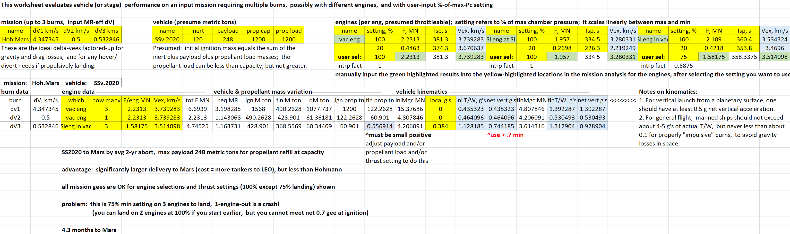
Figure 3 – Faster Transfer With Max Payload, Refilling to Capacity On-Orbit

Figure 4 – Hohmann Transfer With 150 Ton Payload, Minimum Refill On-Orbit

Figure 5 – Faster Transfer With 150 Ton Payload, Minimum Refill On-Orbit
#1. 5-25-20, 2020 Reverse-Engineering Estimates for
Starship/Superheavy Estimates
#2. 9-26-19, Reverse-Engineered “Raptor” Engine
Performance
#3. 6-21-20, Starship/Superheavy 2020 Estimates for Mars
#4. 11-21-19,
Interplanetary Trajectories and Requirements
Update 2-10-21:
I created 2 more worksheets to model the possibilities of
return after refilling on Mars with propellants manufactured on Mars. One was for a min-energy Hohmann return, using a full capacity refill, subject to all the same constraints as the
prior analyses. This one allows less
than half the outbound payload capability,
under the same mission constraints,
because the Mars surface departure is more demanding than the Earth
orbit departure. That is the dominant
factor, which is true even though the Earth landing requires less
burn capability than the Mars landing.
There is latitude here to reduce the refill a little below capacity if
we reduce the payload significantly further.
See Figure 6.
The other explores mission feasibility on the faster
2-year-abort trajectory with a full capacity refill on Mars. This option is “feasible” only with a trivial
2-ton payload and a 20% reduction in the course correction burn budget. There are no feasible solutions for reducing
payload further and reducing the propellant load. There might be a feasible solution with a
very low payload and a full capacity refill,
on a faster trajectory than Hohmann,
but not as fast as the 2-year-abort trajectory. See Figure 7.

Figure 6 – Hohmann Return with Full Refill on Mars

Figure 7 – Fast Return with Full Refill on Mars and Reduced
Course Correction Budget
Update 2-15-21:
I created one more worksheet labeled “flt tst SS” for the
flight tests of prototype “Starships” as single stages with 3 sea level “Raptor”
engines. The 3 burns are ascent, flip,
and touchdown. I added little
calculation blocks to estimate the mass ratio-effective dV requirements for
each.
For the ascent, I
used 1 km/s velocity at 10 km altitude,
and used a Cartesian combination to estimate the combined mechanical
energy, and convert it to velocity at
zero altitude. Because the uncertainty
is enormous, I used a factor of 2
against this speed for the mass ratio-effective value.
For the flip, I
simply guessed a time to accomplish this at a chosen thrust level, on two engines. That gave a total impulse value, which divided by specific impulse, is a propellant mass expended for the
maneuver. Ignoring the touchdown, I combined this propellant mass with the
inert and (zero) payload masses to get a mass ratio for the flip. That and the exhaust velocity get you a dV
with the rocket equation. It is very
approximate at best, and certainly
dominated by the guess for time-to-flip.
The touchdown I figured very similarly to what I have done
before: factor up the descent rate as
the mass ratio-effective dV to touch down.
I used the same factor as before:
1.5, although one could easily
argue for a 2 in experimental work. I
did add an average deceleration gee estimate and an estimate of altitude path length
to decelerate, based on V2 =
2 a s, which should be ignored until all
else is converged.
The estimates converged with 3 engines at 100% thrust for
the ascent, 2 engines at 60% for the
flip, and 2 engines at 60% for the
touchdown. For 120 metric ton inert
mass, and no payload, I’m estimating 146 tons of propellant needed
to reach 1 km/s at 10 km altitude, and
then land with essentially dry tanks.
As the takeoff vertical net accelerations show, this vehicle could launch with more
propellant, and still have 0.5 gee net
vertical capability. So, more ambitious test flights could be pursued.
See Figure 8.

Figure 8 – First-Cut Results for “Starship” Flight Tests
Similar to S/N-8 and S/N-9

No comments:
Post a Comment